Functional Data Analysis

An Overview

J. Derek Tucker

jdtuck@sandia.gov

Sandia National Laboratories

June 4, 2024

Outline

• Definition of Functional Data Analysis
  • Examples
• Mathematical Framework
  • FDA vs Multivariate Statistics
  • Summary Statistics
  • Data Representations
  • Smoothing Functional Data
• Alignment of Functional Data
  • Elastic Method
• Functional Principal Component Analysis
  • Vertical
  • Horizontal
• Modeling

References

• “Functional Data Analysis”, By James Ramsay, B. W. Silverman
• Standard Textbook covers basic methods with a basis-based approach

References

• “Functional and Shape Data Analysis”“, By Anuj Srivastava, Eric P Klassen
• Recent book on advances using more theoretical foundations

Introduction

• Problem of statistical analysis of function data (FDA) is important in a wide variety of applications
• Easily encounter a problem where the observations are real-valued functions on an interval, and the goal is to perform their statistical analysis
• By statistical analysis we mean to compare, align, average, and model a collection of random observations

Canadian Weather

Female Growth

iPhone Bike

Introduction

• Questions then arise on how can we model the functions
  • Can we use the functions to classify diseases?
  • Can we use them as predictors in a regression model
  • It is the same goal (questions) of any area of statistical study
• One problem occurs when performing these type of analyses is that functional data can contain variability in time (\(x\)-direction) and amplitude (\(y\)-direction)
• How do we account for and handle this variability in the models that are constructed from functional data

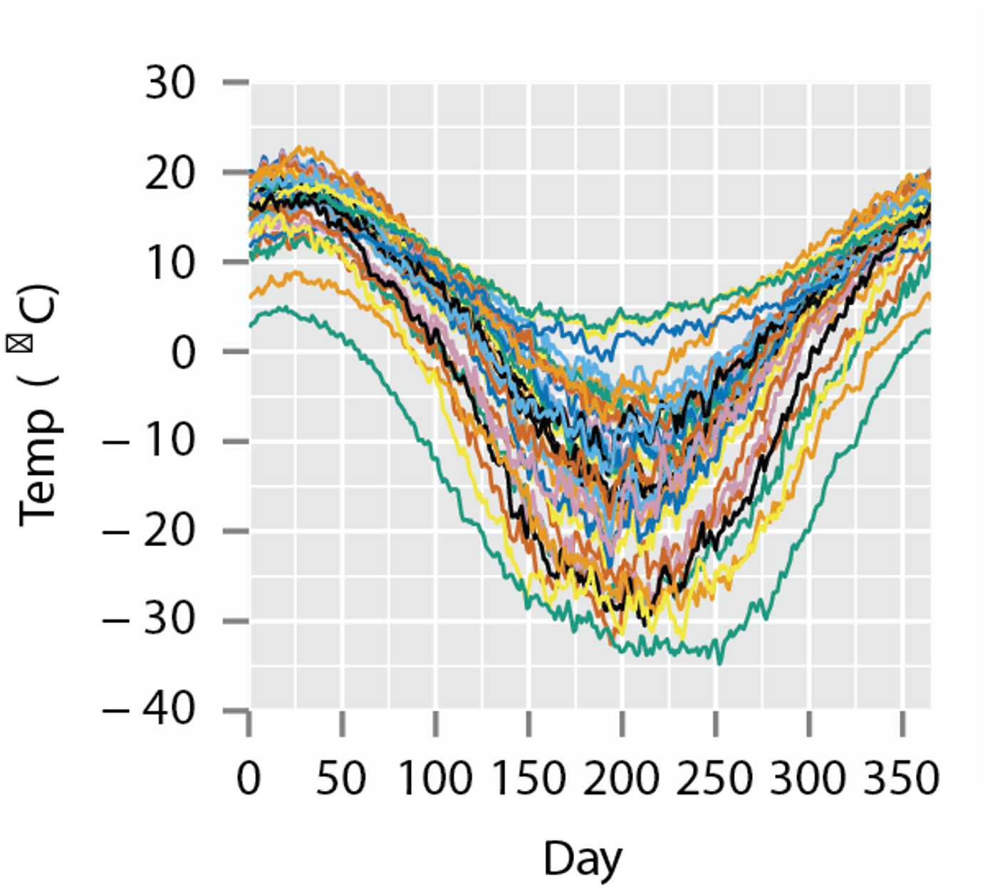
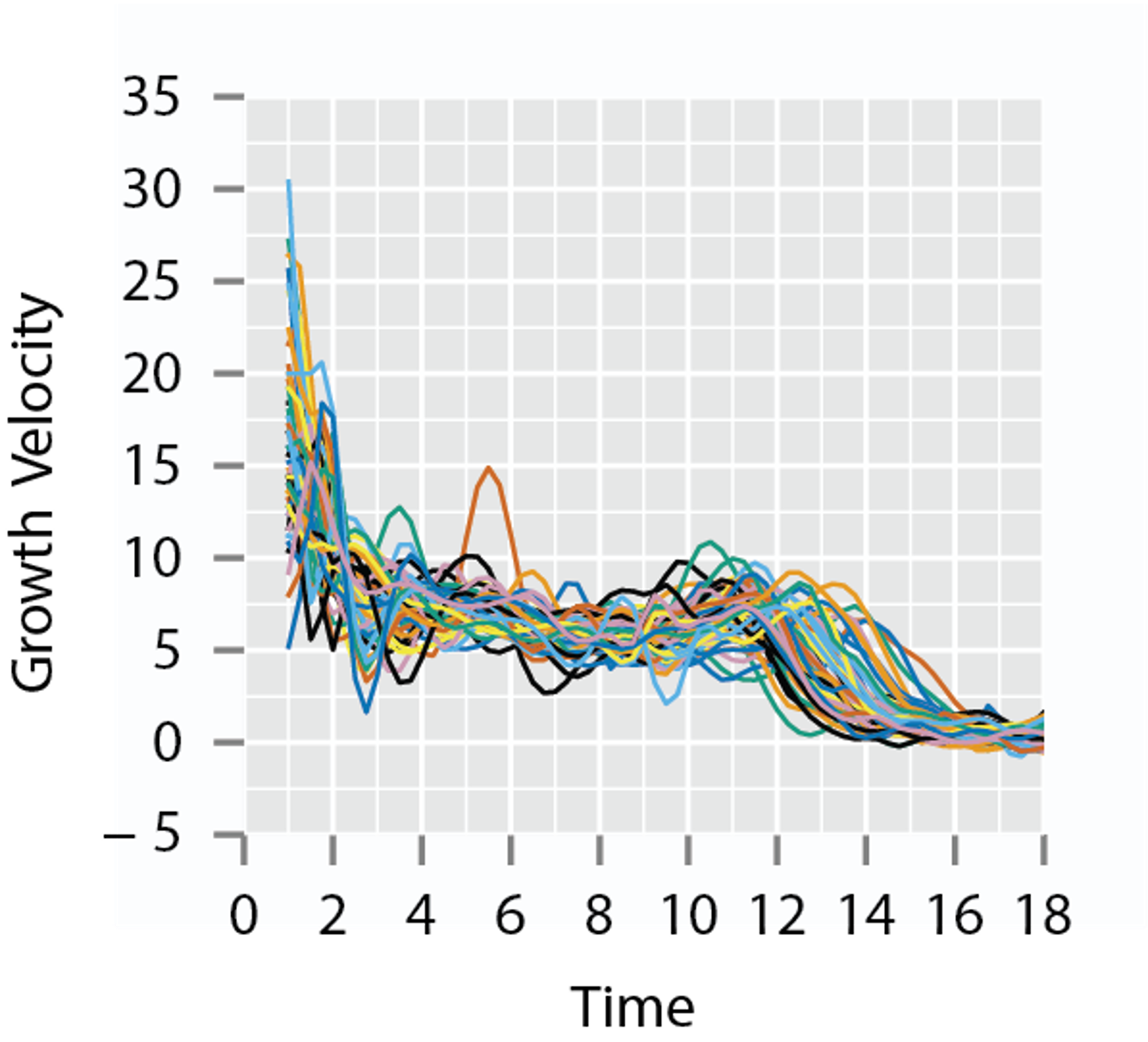
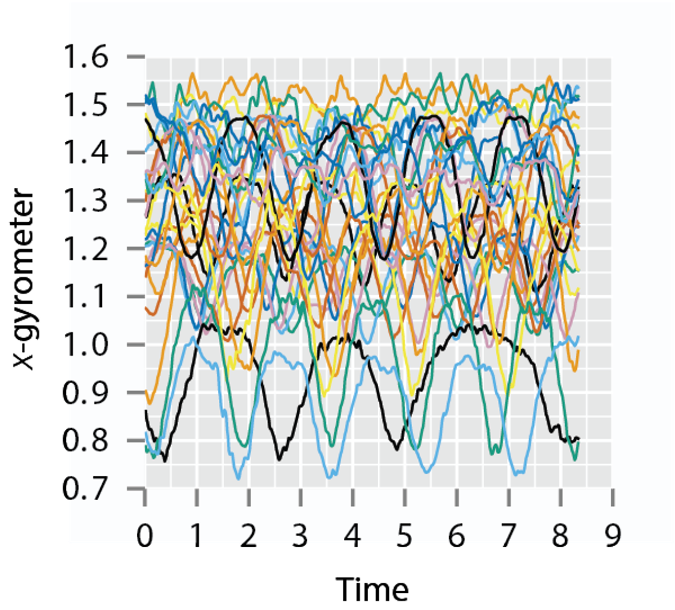
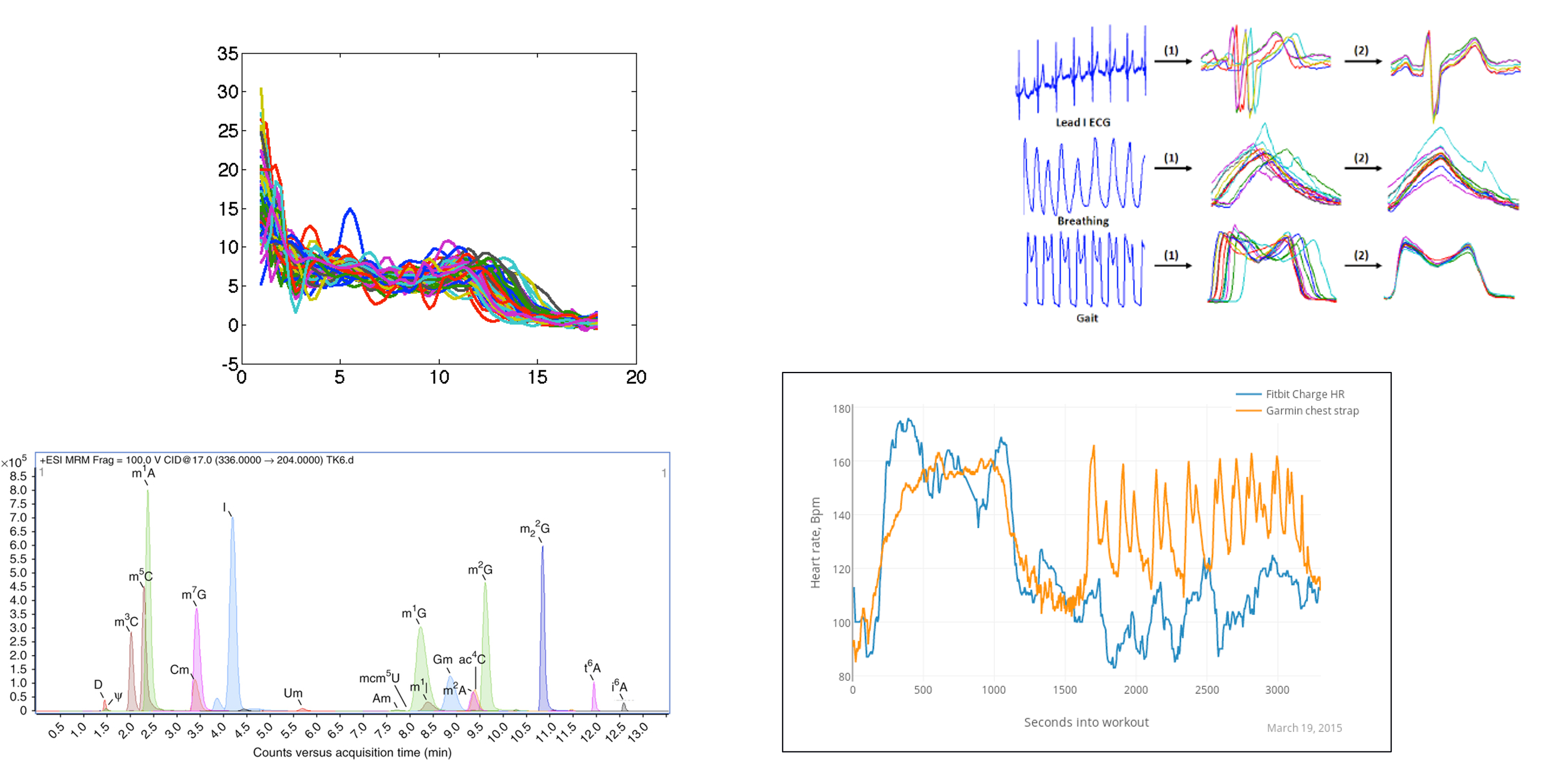
Types of Functional Data

• Real-valued functions, with interval domain: \(f:[a,b]\rightarrow\mathbb{R}\)

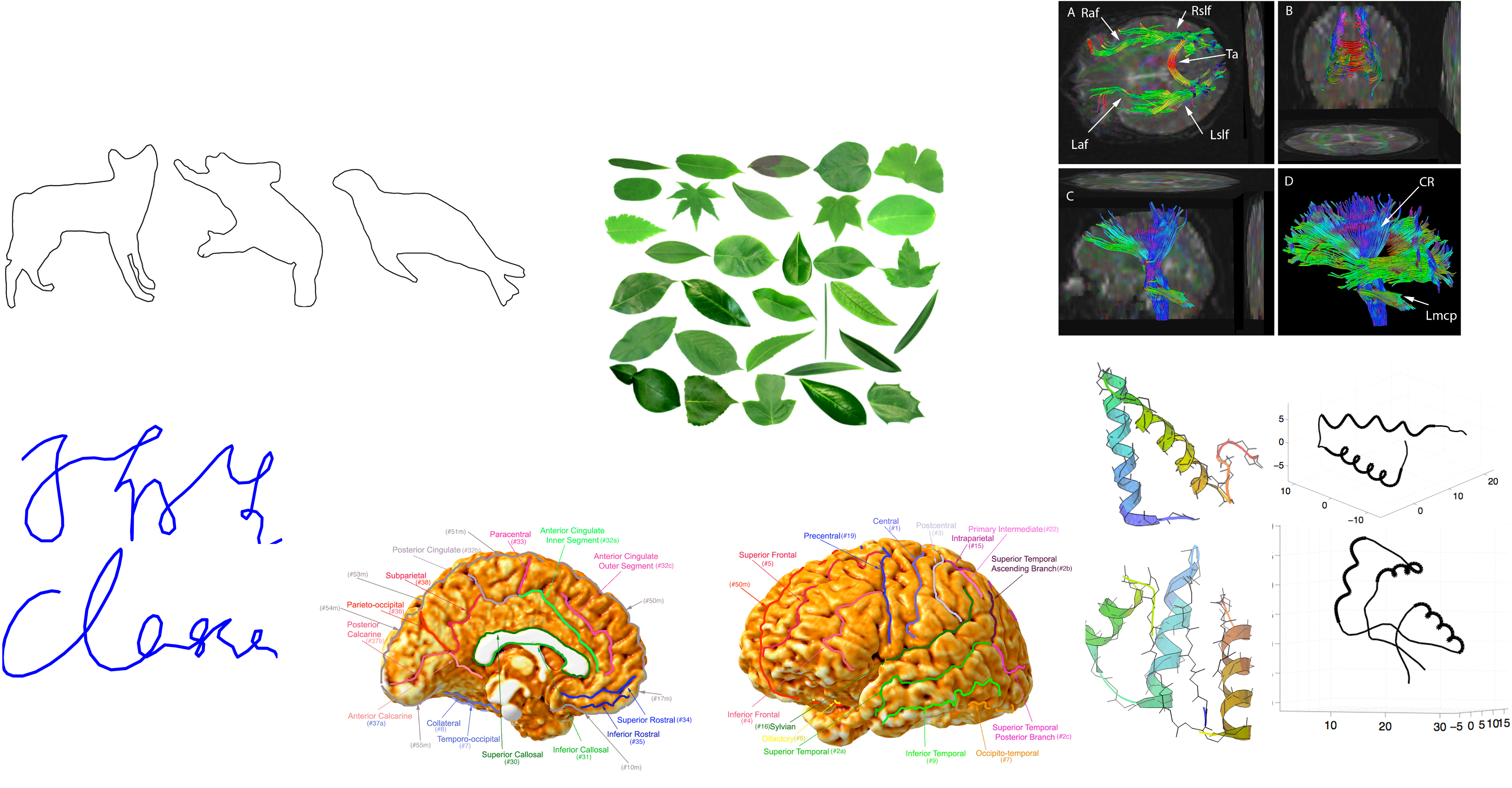
Types of Functional Data

• \(\mathbb{R}^n\)-valued functions with interval domain, Or Parameterized Curves: \(f:[a,b]\rightarrow\mathbb{R}^n\) \(f:S^1\rightarrow\mathbb{R}^n\)

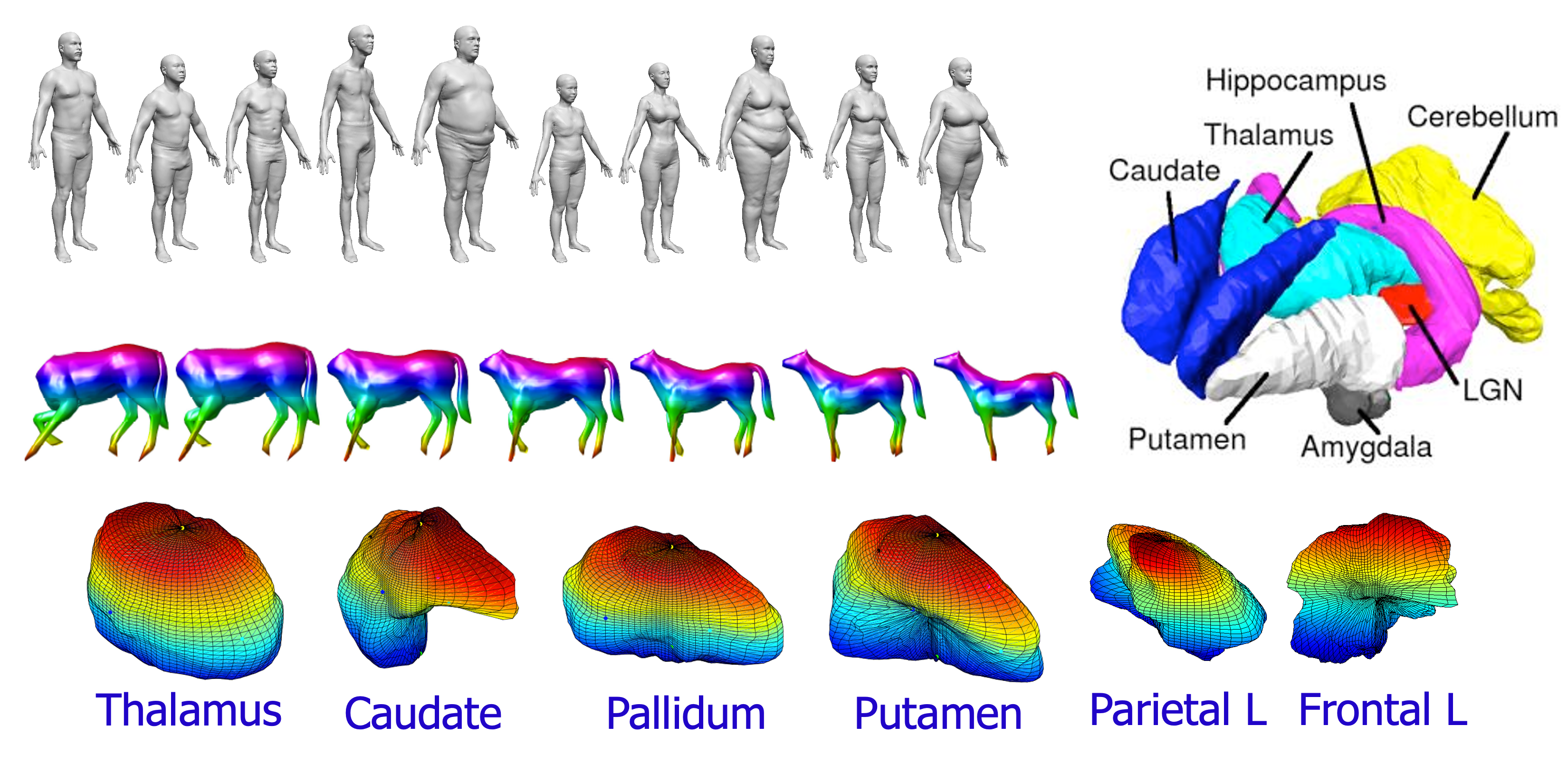
Types of Functional Data

• \(\mathbb{R}^3\)-R3-valued functions on a spherical domain, Or Parameterized Surfaces: \(f:S^2\rightarrow\mathbb{R}^3\)

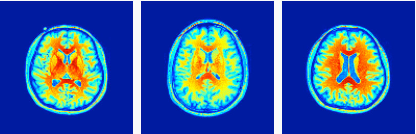
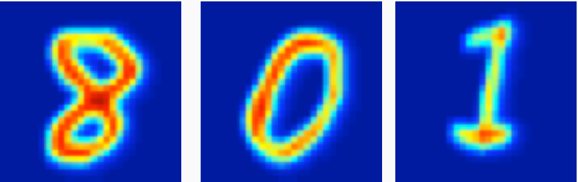
Types of Functional Data

• \(\mathbb{R}^n\)-valued functions with square or cube domains, Or Images: \(f:[0,1]^2\rightarrow\mathbb{R}^n\)

FDA Versus Multivariate Statistics

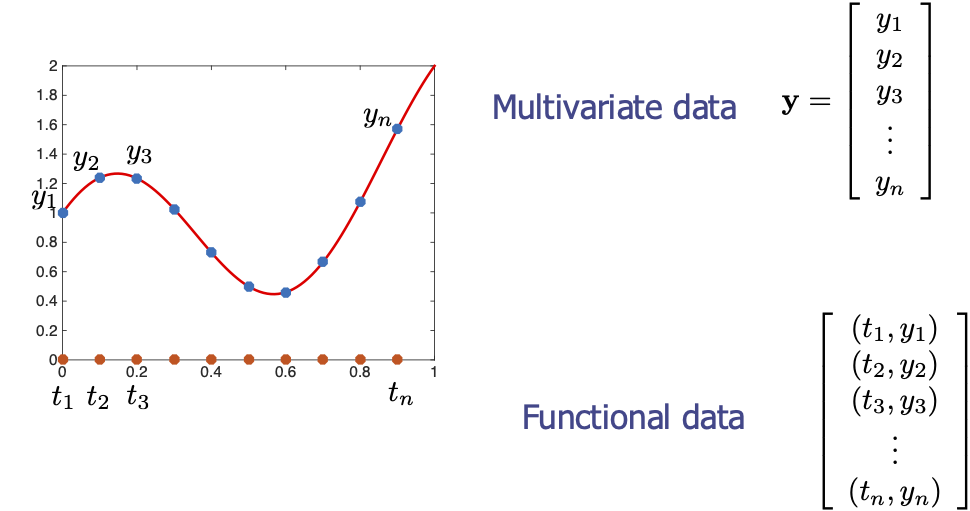
• Not all observations will have the same time indices
• Even if they do, we want the ability to change time indices

FDA Versus Multivariate Statistics

FDA Versus Multivariate Statistics

FDA Versus Multivariate Statistics

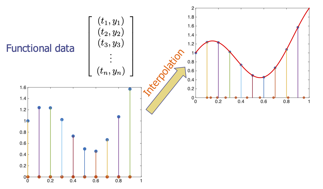
• In FDA, one develops the on function spaces and not finite vectors, and discretizes the functions only at the final step – computer implementation.

• Ulf Grenander: “Discretize as late as possible” (1924-2016)
• Even after discretization, we retain the ability to interpolate resample as needed!

Common Metric Structure for FDA

• Let \(f\) be a real-valued function with the domain \([0,1]\), can be extended to any domain
  • Only functions that are absolutely continuous on \([0,1]\) will be considered
• The \(\mathbb{L}^2\) inner-product: \[\left\langle f_1,f_2 \right\rangle = \int_0^1 f_1(t)f_2(t)\,dt\]
• \(\mathbb{L}^2\) distance between functions: \[ ||f_1-f_2|| = \sqrt{\int_0^1 (f_1(t)-f_2(t))^2\,dt}\]
• From these we will build summary statistics, but how good are they?

Summary Statistics

• Assume that we have a collection of functions, \(f_i(t)\), \(i=1,\dots,N\) and we wish to calculate statistics on this set
• \[\bar{f}(t) = \frac{1}{N}\sum_{i=1}^N f_i(t)\]
• \[\mathop{\mathrm{var}}(f(t)) = \frac{1}{N-1}\sum_{i=1}^N \left(f_i(t) - \bar{f}(t)\right)^2\]
• and the standard deviation function is the point-wise square root of the variance function

Summary Statistics

• The covariance function summarizes the dependence of functions across different time values and is computed for all \(t_1\) and \(t_2\) \[\mathop{\mathrm{cov}}_f(t_1,t_2) = \frac{1}{N-1} \sum_{i=1}^N \left(f_i(t_1) - \bar{f}(t_1)\right)\left(f_i(t_2) - \bar{f}(t_2)\right)\]
• The correlation function is then computed using \[\mathop{\mathrm{corr}}_f(t_1,t_2) = \frac{\mathop{\mathrm{cov}}_f(t_1,t_2)}{\sqrt{\mathop{\mathrm{var}}(f(t_1))\mathop{\mathrm{var}}(f(t_2))}}\]
• Note: These all assume the functions are aligned in time, if not analysis will be affected
  • More on this later…

Smoothing Functional Data

• As assumed earlier the construction of functional observations, \(f_i\) is done using discrete data (implementation)
• In some situations, the signal-to-noise ration is low, or the data is noisy, or the discrete observations are few in number
  • Can cause problems in generating sufficient summary statistics
  • It can be essential to use information in neighboring or similar functions to get better estimates
• The following methods help solve this problem

Representing Functions by Basis Functions

• We can represent a function by a set of basis functions, \(\theta_i\), \(i=1,\dots,k\)
• Basis Types
  • Fourier
  • B-Spline
• We can represent a function \(f\) by a linear expansion \[f(t) = \sum_{i=1}^p b_i \theta_i\]
• in terms of \(p\) basis functions \(\theta_i\) and coefficients \(b_i\)
• Find the basis coefficients, \(b_i\) by minimizing the least-squares \[{\mathbf b}^* = \mathop{\mathrm{arg\,min}}_{{\mathbf b}}({\mathbf f}- \Theta{\mathbf b})^{\mathsf{T}}({\mathbf f}-\Theta{\mathbf b})\]

Representing Functions by Basis Functions

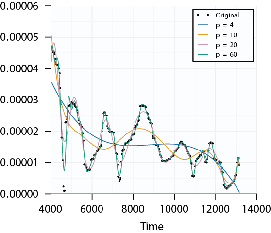
• Setting the dimension of the basis expansion \(p\) we can control the degree to which the functions are smoothed
• Choosing \(p\) large enough we can fit the data well, but might fit any additive noise

Kernel Smoothing

• Another type of smoothing of functional data is kernel smoothing
• The smooth function \(\hat{f}(t)\) is computed at a given point and is a linear combination of local observations \[ \hat{f}(t) = \sum_{i=1}^n S_j(t) f(t_j)\]
• An example of \(S(t)\) is the Nadaraya-Watson estimator \[ S_j(t) = \frac{\mathop{\mathrm{Kern}}[(t_j-t)/h]}{\sum_r\mathop{\mathrm{Kern}}[(t_r-t)/h]}\]
• where \(\mathop{\mathrm{Kern}}\) is a kernel function obeying Mercer’s conditions and \(h\) is the bandwidth of the kernel

Roughness Penalty

• Another popular way to smooth functional data is to add a roughness penalty to the least-squares fit
• The way to quantify the notion of roughness is the square of the second derivative, \([D^2 f(t)]^2\) which is also known as the curvature at \(t\)
• A natural measure of a function’s roughness is the integrated squared second derivative \[ \mathop{\mathrm{pen}}(f) = \int [D^2 f(t)]^2\,dt\]
• Can define a compromise that trades of smoothness against data fit of a basis using the penalized least-squares fit \[ {\mathbf b}^* = \mathop{\mathrm{arg\,min}}_{{\mathbf b}}({\mathbf f}- \Theta{\mathbf b})^{\mathsf{T}}({\mathbf f}-\Theta{\mathbf b})+ \lambda \mathop{\mathrm{pen}}(\Theta{\mathbf b})\]

Roughness Penalty

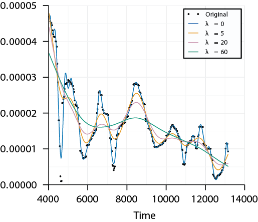
• The parameter \(\lambda\) is the smoothing parameter and controls the amount of smoothing

Functional Principal Component Analysis

• The motivation for functional principal component analysis (fPCA) is that the directions of high variance will contain more information then direction of low variance
• The optimization problem for fPCA \[\min_{w_i} E\|f-\hat{f}\|^2\]
• where \(\hat{f} = \mu_f + \sum_{i=1}^n \beta_i w_i(t)\) is the fPCA approximation of \(f\)
• We then use the sample covariance function \(\mathop{\mathrm{cov}}(t_1,t_2)\) to form a sample covariance matrix \(K\)
• Taking the SVD, \(K=U\Sigma V^{\mathsf{T}}\) we can calculate the directions of principle variability in the given functions using the first \(p\leq n\) columns of \(U\)

Functional Regression

• In functional data analysis, regression modeling is where the function variables are used as predictors to estimate a scalar response variable
• Standard functional linear regression model \[ y_i = \alpha + \int_0^T f_i(t)\beta(t)\,dt+\epsilon_i,~~i=1,\dots,n\]
• where \(\alpha \in \mathbb{R}\) is the intercept, \(\beta(t)\) is the regression-coefficient function and \(\epsilon_i \in \mathbb{R}\) are random errors
• The model parameters are usually estimated by minimizing the sum of squared errors (SSE) \[ \{\alpha^*,\beta^*(t)\} = \mathop{\mathrm{arg\,min}}_{\alpha,\beta(t)} \sum_{i=1}^n |y_i - \alpha - \int_0^T f_i(t)\beta(t)\,dt|^2\]

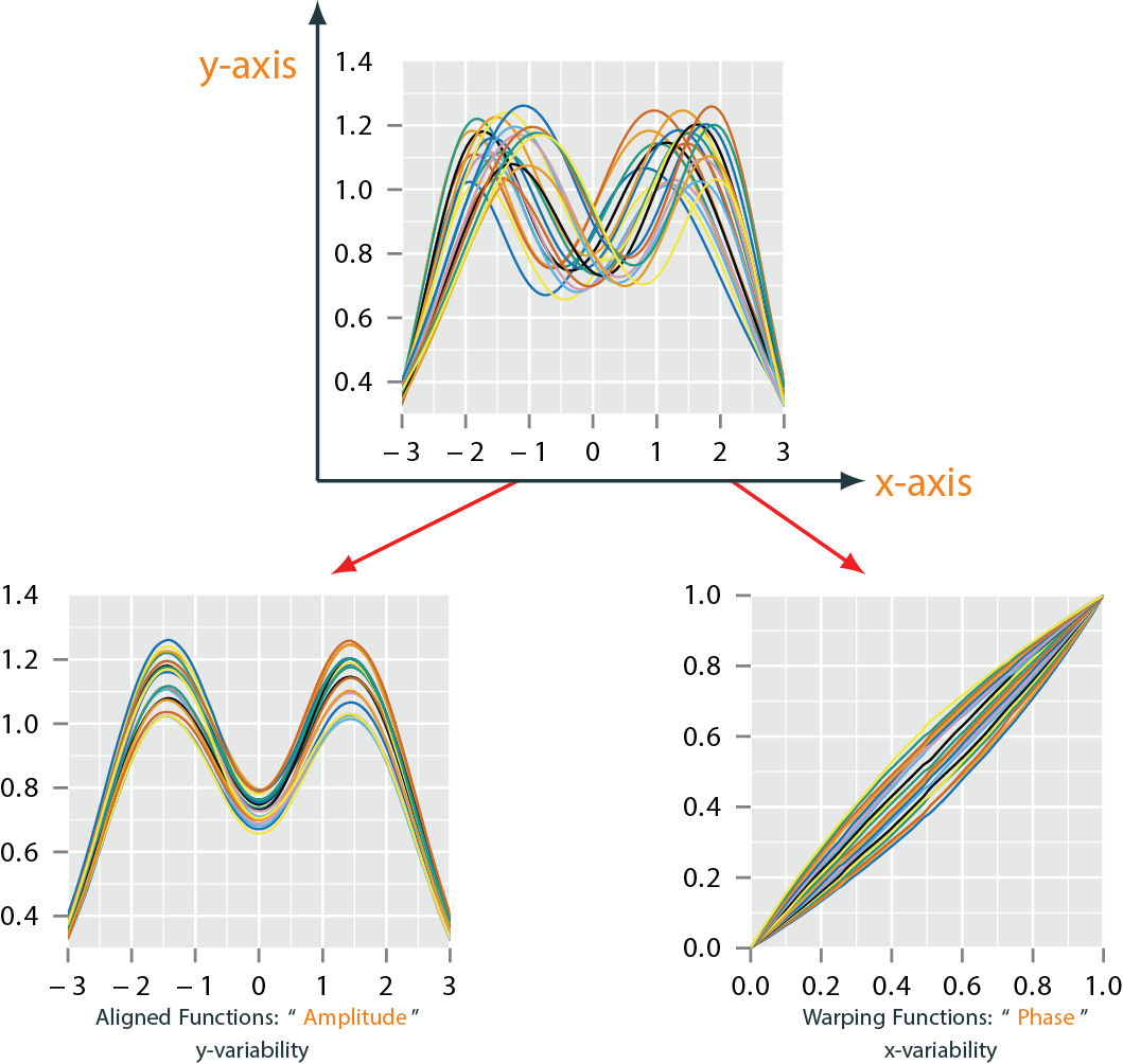
Phase Amplitude Separation

• All of these methods assume the data has no phase-variability or is aligned
• How does this affect the analysis?
• Can we account for it?

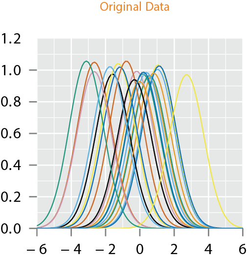
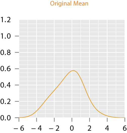
Motivation

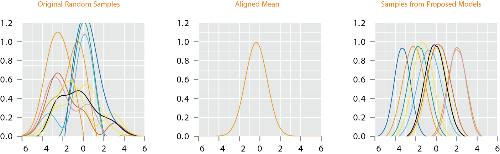
• If one performs fPCA on this data and imposes the standard independent normal models on fPCA coefficients, the resulting model will lack this unimodal structure
• A proper technique is to incorporate the phase and amplitude variability, into the model construction which in turn incorporates into the component analysis

Functional Data Alignment

Functional Data Alignment

• There are few different methods that have been proposed (Ramsay, Mueller, Srivastava)
• We will focus on Elastic Method of (Srivastava, Wu, Tucker, Kurtek) as it uses a proper metric
• Let elements of the group \(\Gamma\) play the role of warping functions as the set of boundary-preserving diffeomorphisms, \(\gamma: [0,1] \to [0,1]\)
• For any \(f\), the operation, \(f\circ\gamma\) denotes the time warping of \(f\) by \(\gamma\)

Functional Data Alignment

• Problem: Under the standard \({\mathbb{L}^2}\) metric,
  • The action of \(\Gamma\) does not act by isometries since \(\| f_1\circ \gamma - f_2 \circ \gamma\|\neq\| f_1 - f_2 \|\)
• Solutions:
  • Use the square-root slope function or SRSF of \(f\) \[ q(t) = \mbox{sign}(\dot{f}(t)) \sqrt{ |\dot{f}(t)|} \]
• where \(\| q_1 - q_2 \| = \| (q_1, \gamma) - (q_2, \gamma) \|\) and \((q_1, \gamma) = (q_1 \circ \gamma)\sqrt{\dot{\gamma}}\)
• Leads to a distance on \({\mathcal F}/ \Gamma\): \(d_a(f_1, f_2) = \inf_{\gamma \in \Gamma} \|q_1 - (q_2,\gamma)\|\)

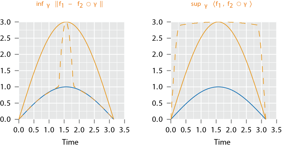
Pinching Problem

• Why use the ?
  • The \({\mathbb{L}^2}\) distance is a proper distance
  • The action of \(\Gamma\) does act by isometries
  • Solves the pinching problem

Elastic Function Alignment

• Alignment:
  1. Alignment is performed by finding the empirical Karcher mean \[ \mu_q = \mathop{\mathrm{arg\,min}}_{q \in {\mathbb{L}^2}} \sum_{i=1}^n \left( \inf_{\gamma_i \in \Gamma} \| q - (q_i, \gamma_i) \|^2 \right)\]
  2. Note that if \({\mu}_q\) is a minimizer of the cost function, then so is \(({\mu}_q ,\gamma)\) for any \(\gamma \in \Gamma\) since the metric is invariant to random warpings
  3. To make the choice unique we choose the \(\mu_q\) of the set \(\{ (\mu_q,\gamma) | \gamma \in \Gamma\}\) such that the mean of \(\{\gamma_i^*\}\) is identity

Elastic Function Alignment

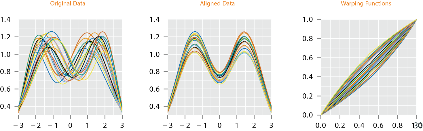
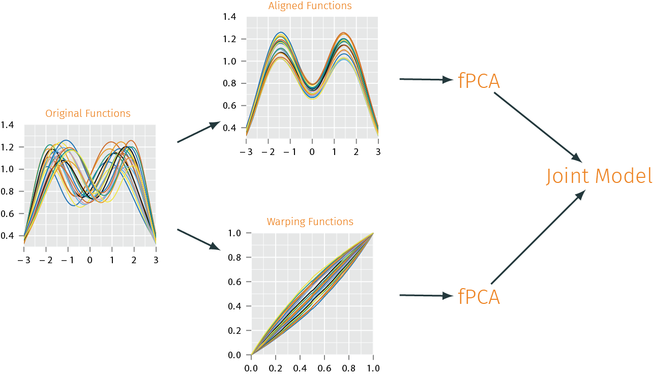
Modeling using Phase & Amplitude Separation

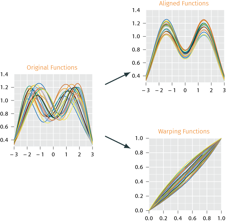
Modeling using Phase & Amplitude Separation

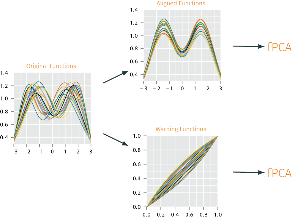
Modeling using Phase & Amplitude Separation

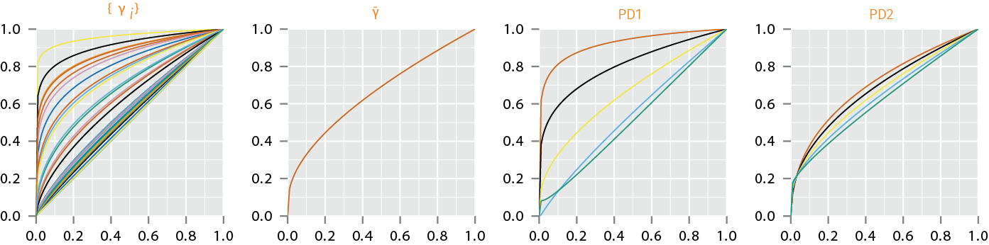
Analysis of Warping Functions (Phase)

• Horizontal fPCA: Analysis of Warping Functions
  • Use SRSF of warping functions, \(\psi = \sqrt{\dot{\gamma}}\)
  • Karcher Mean: \(\gamma \mapsto \sum_{i=1}^n d_p(\gamma, \gamma_i)^2\)
  • Tangent Space:\(T_{\psi}({\mathbb{S}}_{\infty}) = \{v \in {\mathbb{L}^2}| \int_0^1 v(t) \psi(t) dt = 0\}\)
  • Sample Covariance Function: \((t_1, t_2) \mapsto \frac{1}{n-1} \sum_{i=1}^n v_i(t_1) v_i(t_2)\)
  • Take SVD of \(K_{\psi} = U_{\psi} \Sigma_{\psi} V_{\psi}^{\mathsf{T}}\) provides the estimated principal components

Why SRSF of \(\gamma_i\)

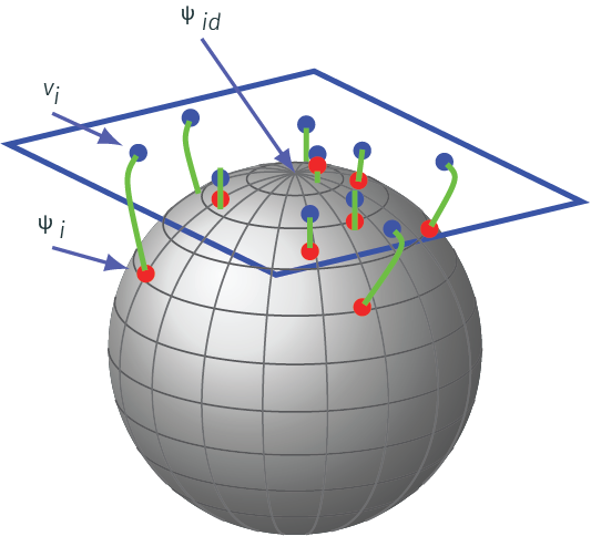
• \(\Gamma\) is a nonlinear manifold and it is infinite dimensional
• Represent an element \(\gamma \in \Gamma\) by the square-root of its derivative \(\psi = \sqrt{\dot{\gamma}}\)
• Important advantage of this transformation is that set of all such \(\psi\)s is a Hilbert sphere \({\mathbb{S}}_{\infty}\)

Analysis of Aligned Functions (Amplitude)

• Vertical fPCA: Analysis of Aligned Functions
  • Need variability associated with the initial values (\(\{f_i(0)\}\))
    • Analyze the aligned pair \(\tilde{h} = [\tilde{q}_i~~f_i(0)]\) such that mapping from the function space \({\mathcal{F}}\) to \({\mathbb{L}^2}\times \mathbb{R}\) is a bijection \[ K_h = \frac{1}{n-1}\sum_{i=1}^n E[(\tilde{h}_i - \mu_h)(\tilde{h}_i - \mu_h)^{\mathsf{T}}] \in \mathbb{R}^{(T+1) \times (T+1)} \]
  • Taking the SVD, \(K_h=U_h\Sigma_h V_h^{\mathsf{T}}\) we can calculate the directions of principle variability

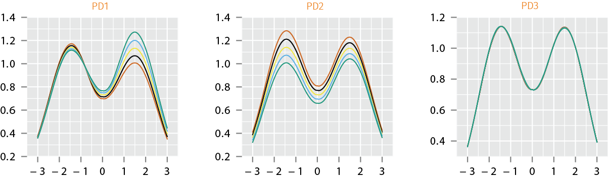
Analysis of Aligned Functions (Amplitude)

Sampling from Joint Model

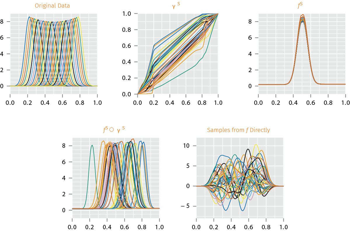
• Random samples from jointly Gaussian models on fPCA coefficients of \(\gamma^s\) and \(f^s\), and their combinations \(f^s \circ \gamma^s\), with samples from \(f\) directly.

Summary

• FDA is a very important problem area for statistics
• Can perform statistics using functions, but have to be aware of different set of issues/nuances
• Functional data often comes with phase variability that cannot be handled using standard L2 framework
• Elastic FDA provides more flexibility than classical FDA
  • Amongst the best alignment methods
  • Also provides joint solutions for inferences along with alignments
• Theory and Methods work for functions, curves, surfaces, and images

Questions?

jdtuck@sandia.gov

http://research.tetonedge.net