Bayesian Model Calibration
An Elastic Approach
J. Derek Tucker, Statistical Sciences
2023-01-24
![]()
Sandia National Laboratories
- Department of Energy National Lab
- 14,000 Staff across 7 Locations
- Two Statistics Departments
- 30 Full Time Staff, 4 Post-Docs, 10 year round interns
Outline
- Introduction
- Functional Data Analysis
- Elastic Metric
- Bayesian Model Calibration
- Results
- Simulation
- Sandia Z-Machine
Introduction
- Question: How can we model functions
- Can we use the functions to classify diseases?
- Can we use them as predictors in a regression model?
- Can we calibrate a computer model?
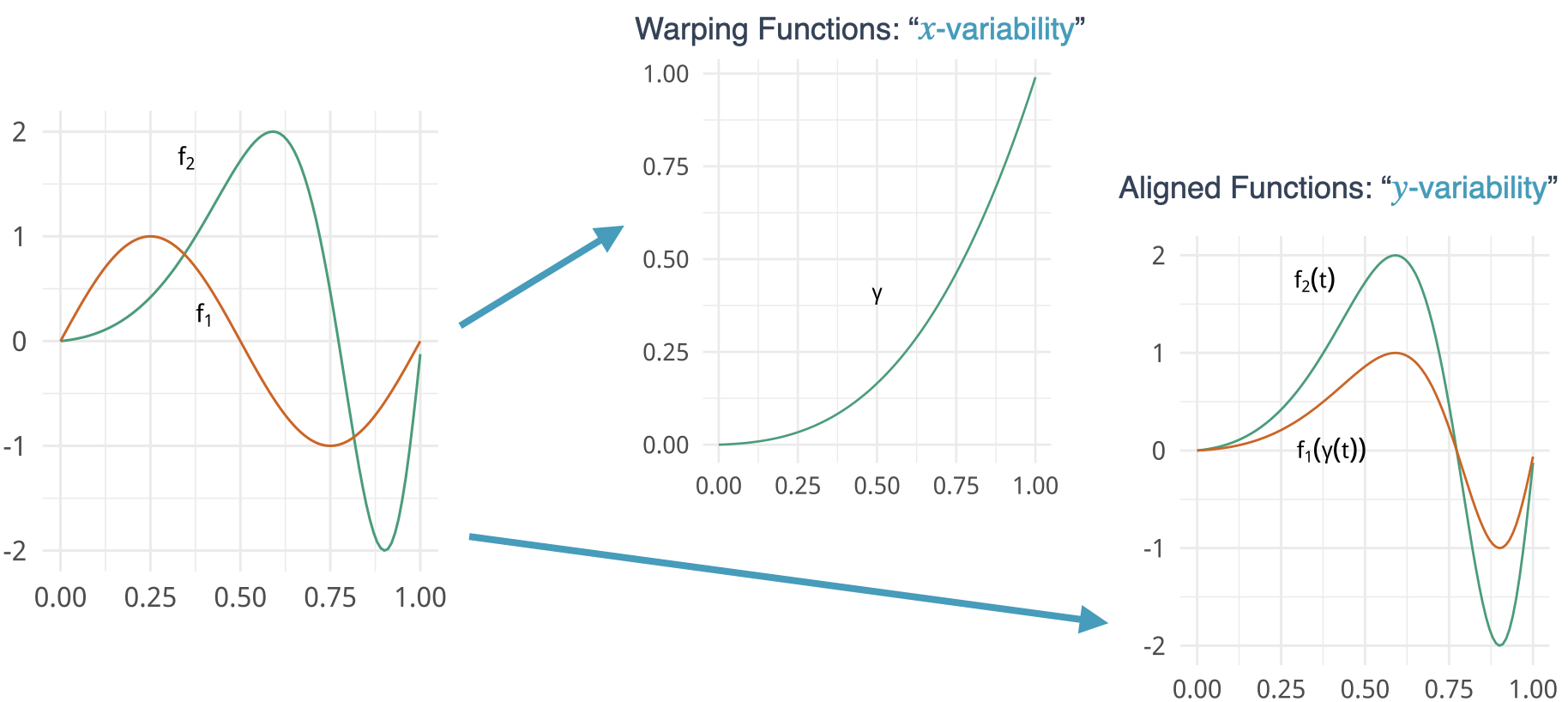
- One problem occurs when performing these types of analysis is that functional data can contain variability in time (x-direction) and amplitude (y-direction)
- How do we characterize and utilize this variability in the models that are constructed from functional data?
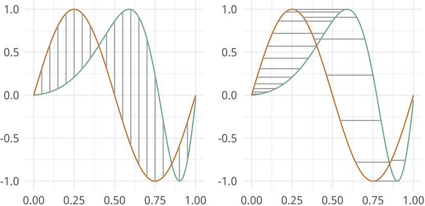
Components of Function Variability
Elastic Distance (Fisher-Rao)
Define the Square Root Velocity Function \[q:[0,1]\rightarrow\mathbb{R}^1,~q(t)=sign(\dot{f}(t))\sqrt{|\dot{f}(t)|}\] Fisher Rao Distance is \(\mathbb{L}^2\) in SRVF space \[d_a(f_1,f_2) = \inf_\gamma\|(q_1\circ\gamma)\sqrt{\dot{\gamma}}-q_2\|\] Distance is a proper distance
Can compute distance on warping functions (how much alignment) \[d_p(\gamma) = \arccos\left(\int_0^1\sqrt{\dot{\gamma}}\,dt\right)\] 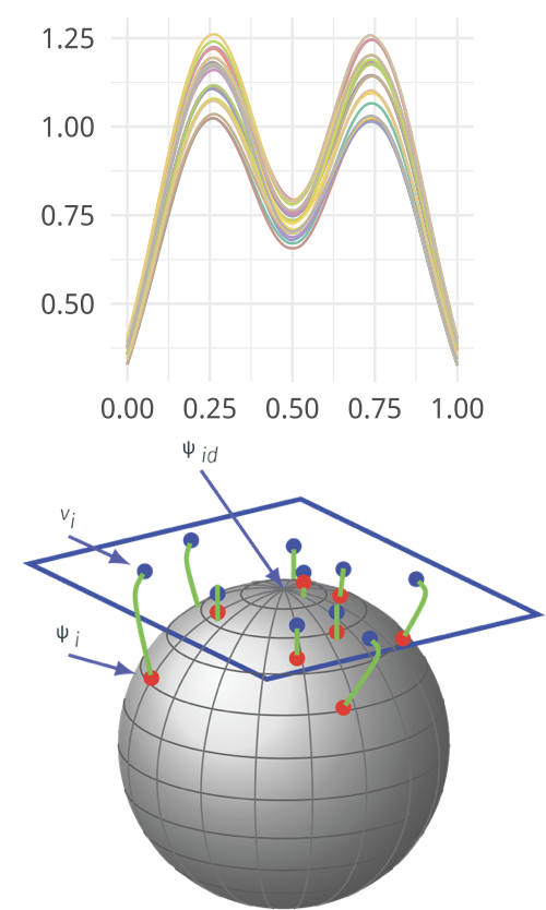
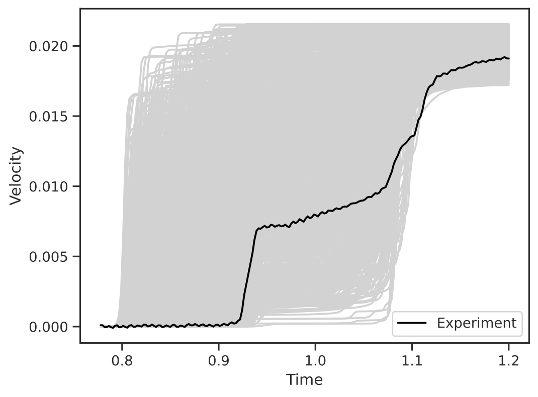
Bayesian Model Calibration
- We wish to calibrate a computer model with parameters \(\theta\) to an experiment
- Can compute computer model (simulations) over wide range of \(\theta\)
- The data is functional in nature and has phase and amplitude variability
- Utilize elastic metrics in a Bayesian Model Calibration Framework
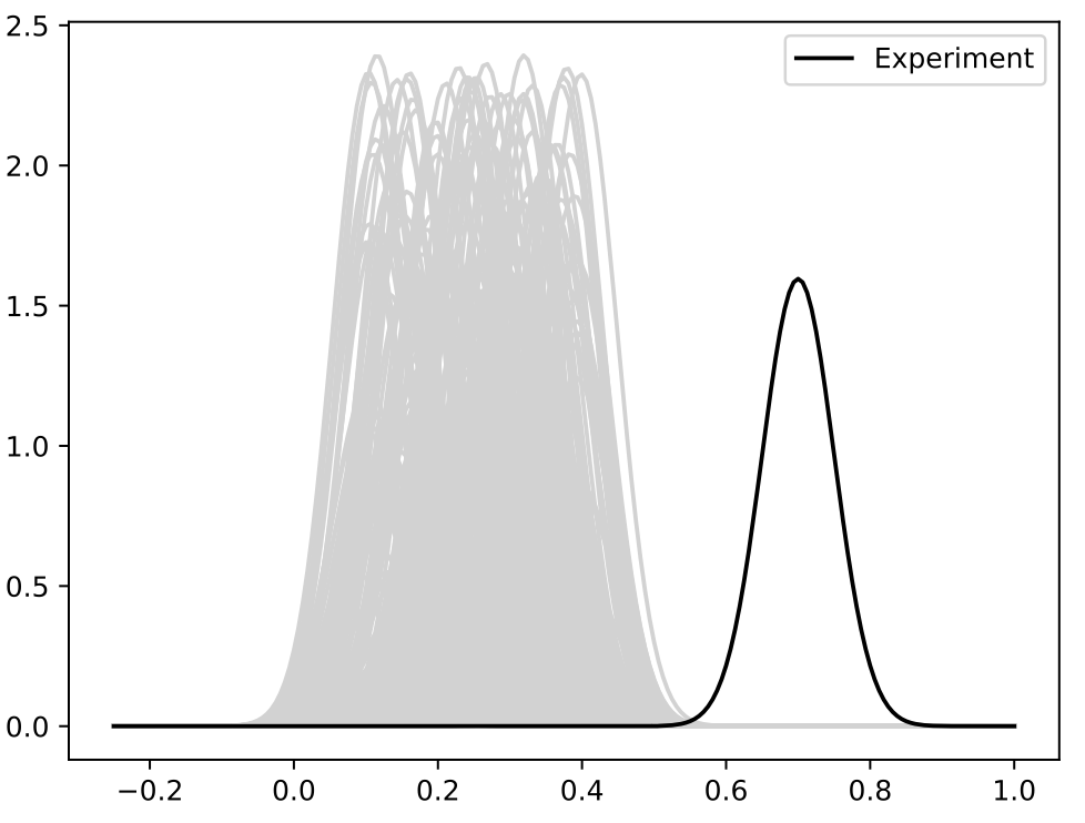
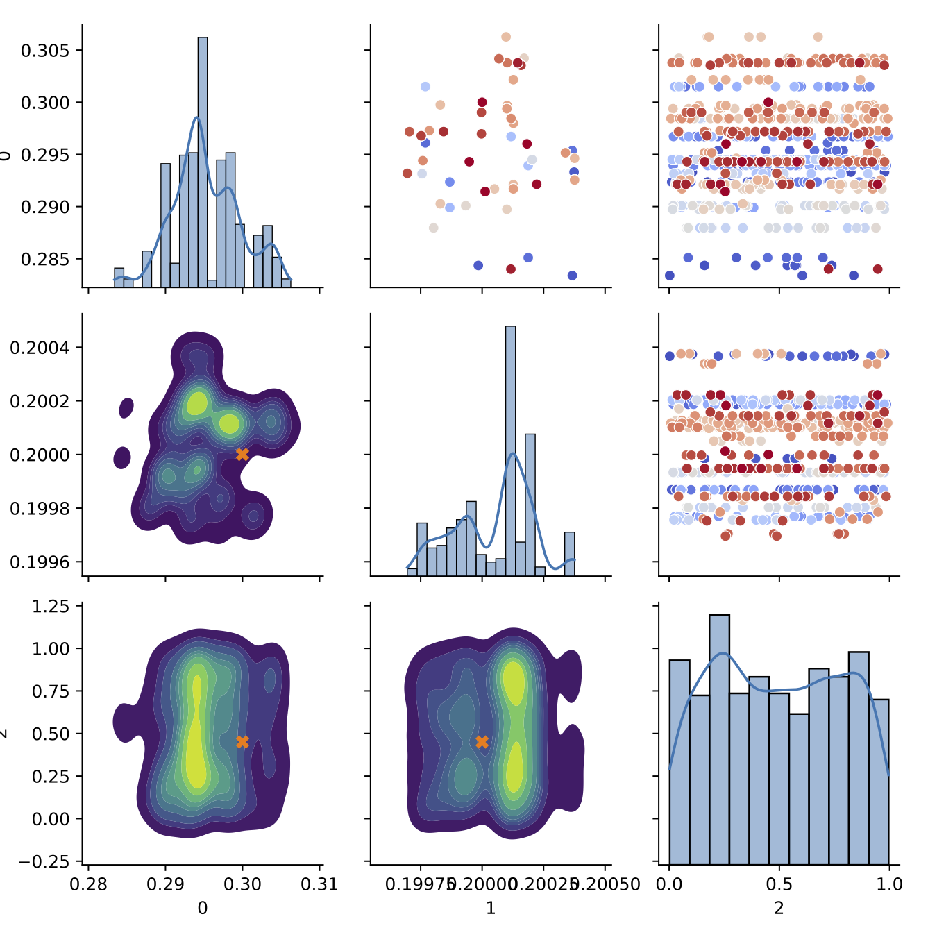
Simulation
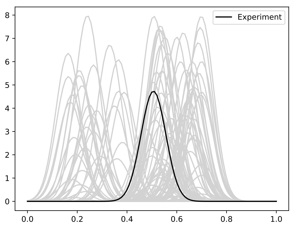
- Simulation study where each function is parameterized Gaussian pdf
- A set of 100 functions were simulated with \(\theta_1,\theta_2\) being drawn from a \(U[0,1]\)
- Third nuisance parameter \(\theta_3\) also drawn from \(U[0,1]\)
\[f_i(t) = \frac{\theta_1}{0.05\sqrt{2\pi}}\exp\left(-\frac{1}{2}\left(\frac{t-(\sin(2\pi \theta_0^2)/4-\theta_0/10+0.5)}{0.05}\right)^2\right)\]
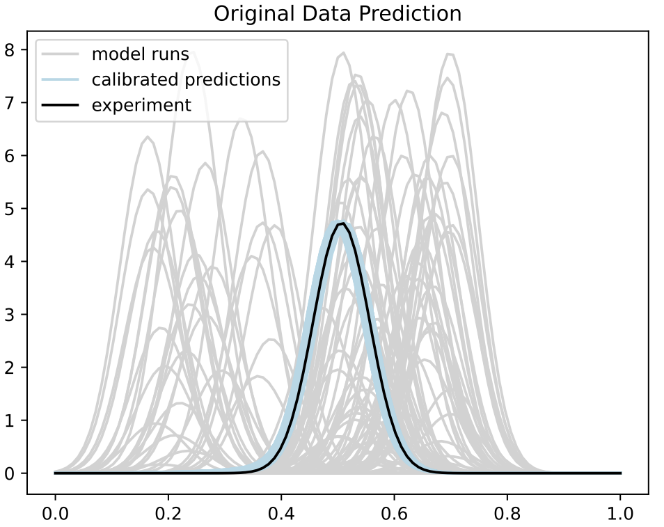
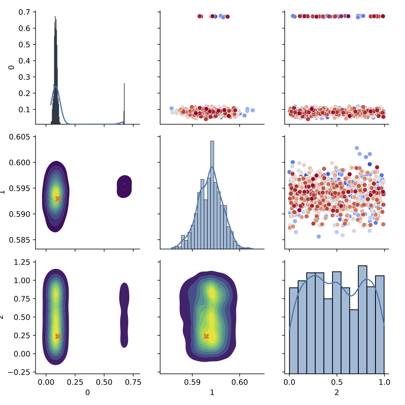
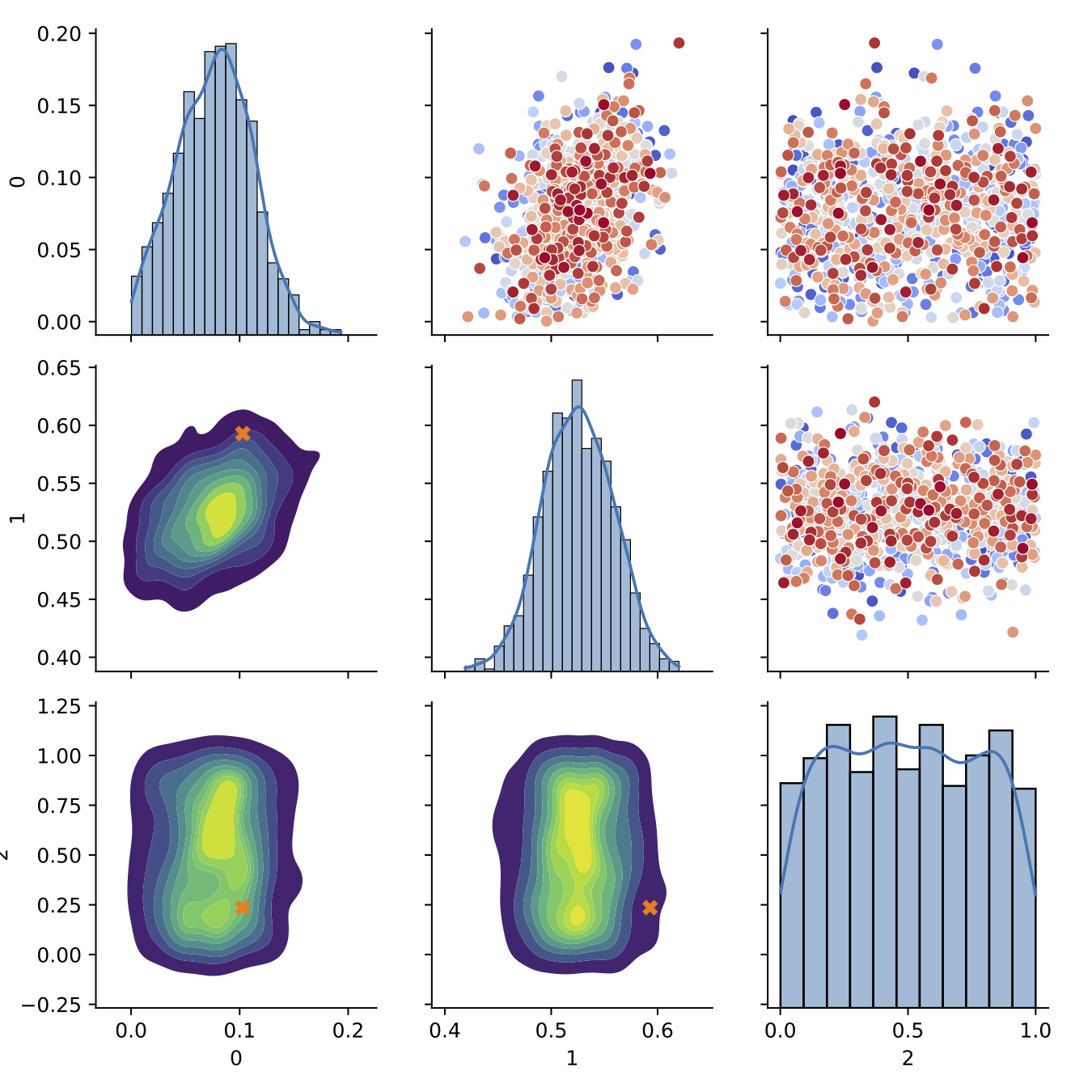
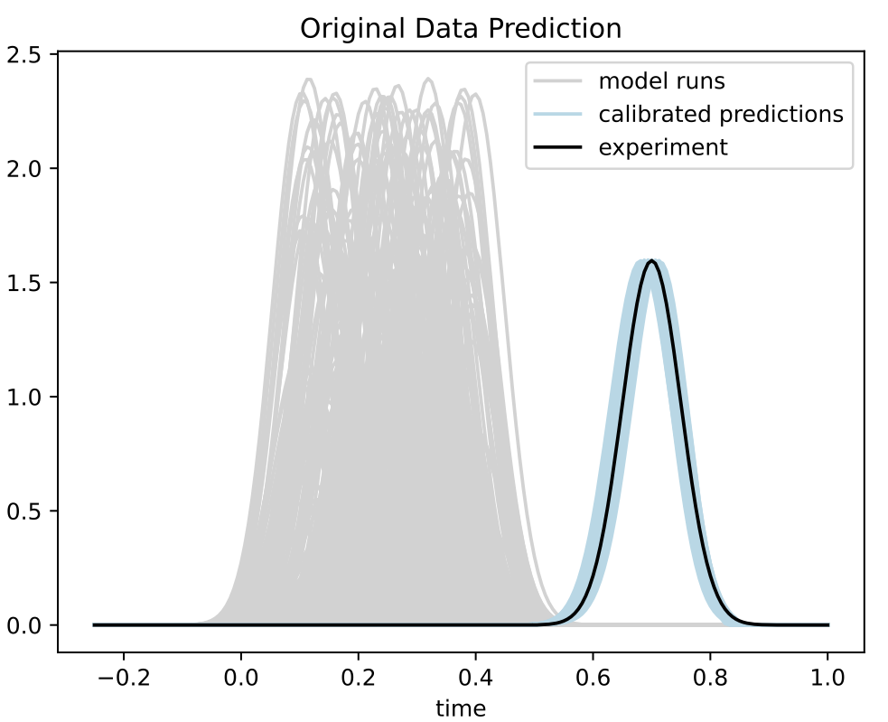
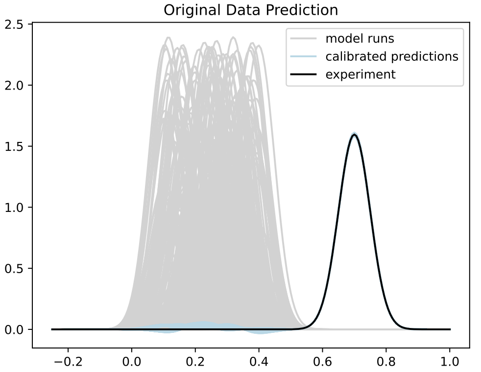
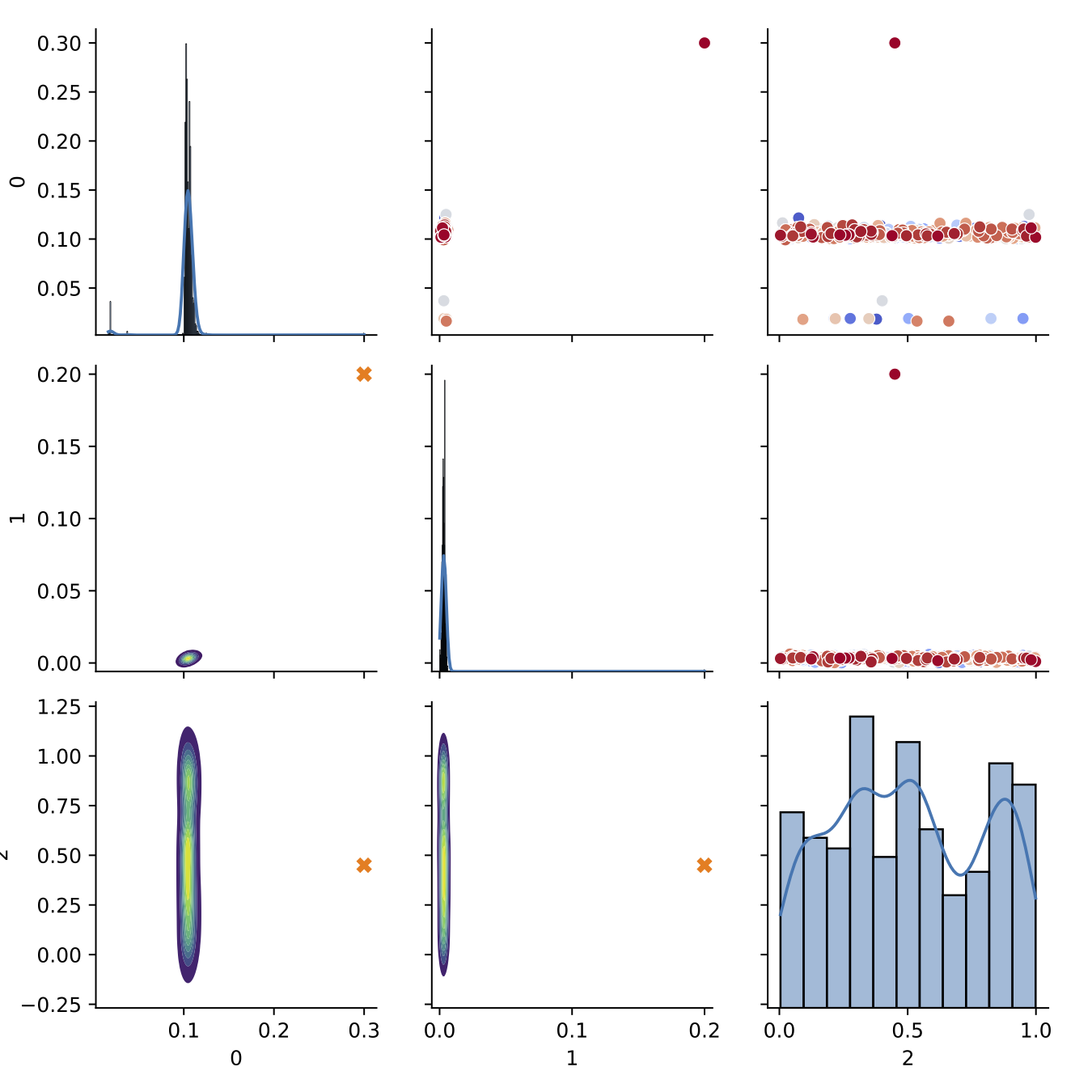
Calibration
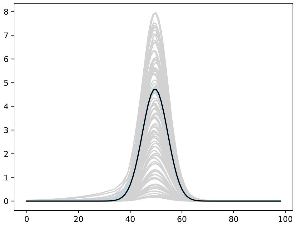
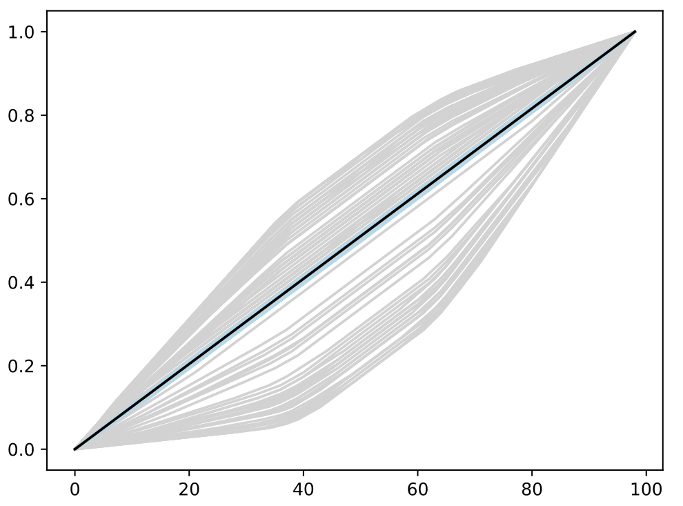
- Trained BASS Emulator on Aligned Functions and Shooting Vectors (using elastic fPCA)
- Calibrated using framework with tempering and adaptive MCMC
- Blue shows draws from posterior distribution at 95% credible interval
Calibration
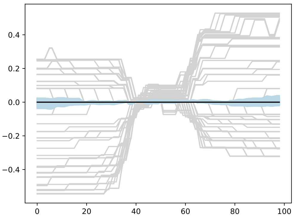
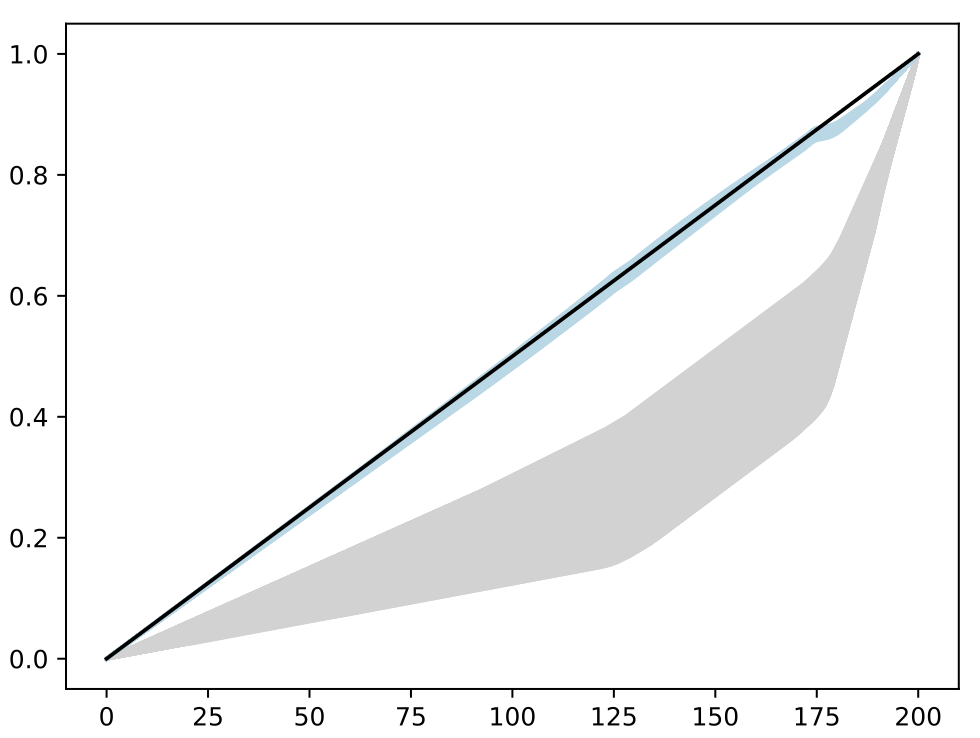
Comparison to Standard Method
Simulation with Discrepancy
- Repeat same simulation model with with the experiment having a timing discrepancy
- Discrepancy modeling with basis functions in shooting vector space
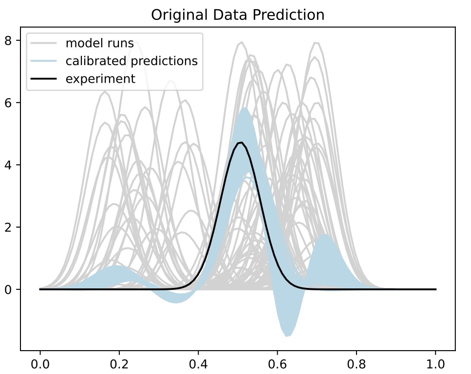
Calibration
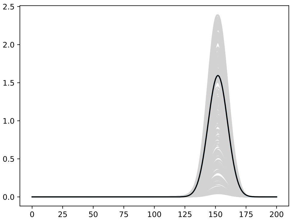
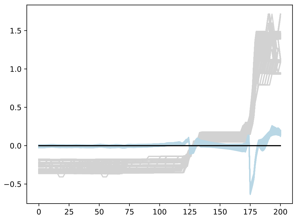
- Trained BASS Emulator on Aligned Functions and Shooting Vectors (using elastic fPCA)
- Calibrated using framework with tempering and adaptive MCMC
- Blue shows draws from posterior distribution at 95% credible interval
Calibration
Comparison to Standard Method
Calibration of Tantalum
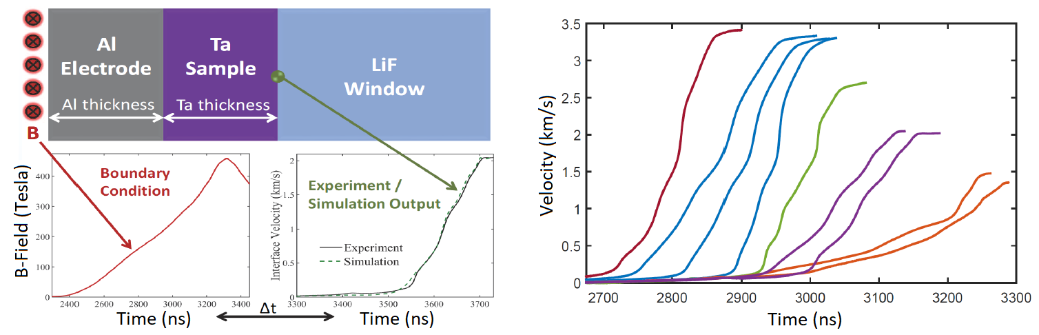
- Calibration equation of state of tantalum generated with pulse magnetic fields
- Estimate the parameters describing the compressibility (relationship between pressure and density) to understand extreme pressures
- Conducted using Sandia Z-machine, a pulse power drive reactor
Calibration
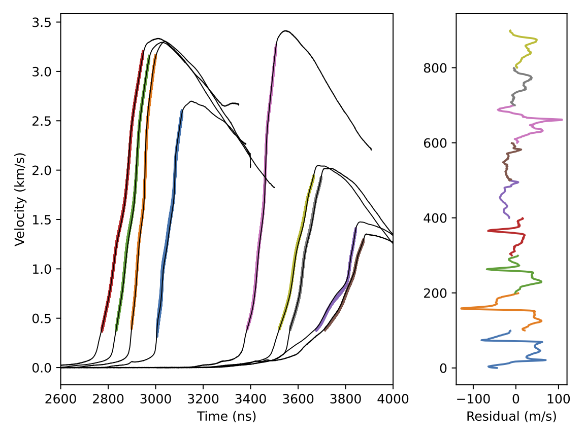
- We have a good fit between experiment and simulation
- Better residuals over standard calibration method
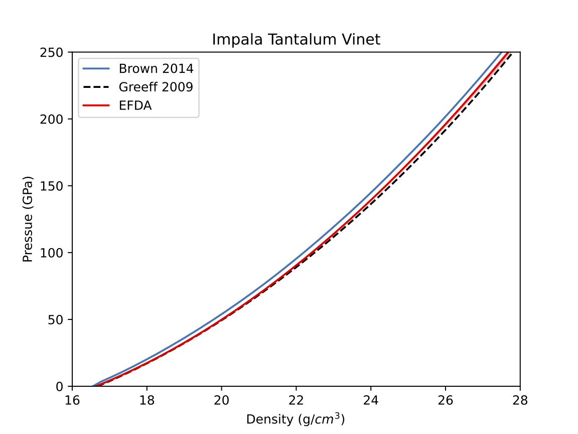
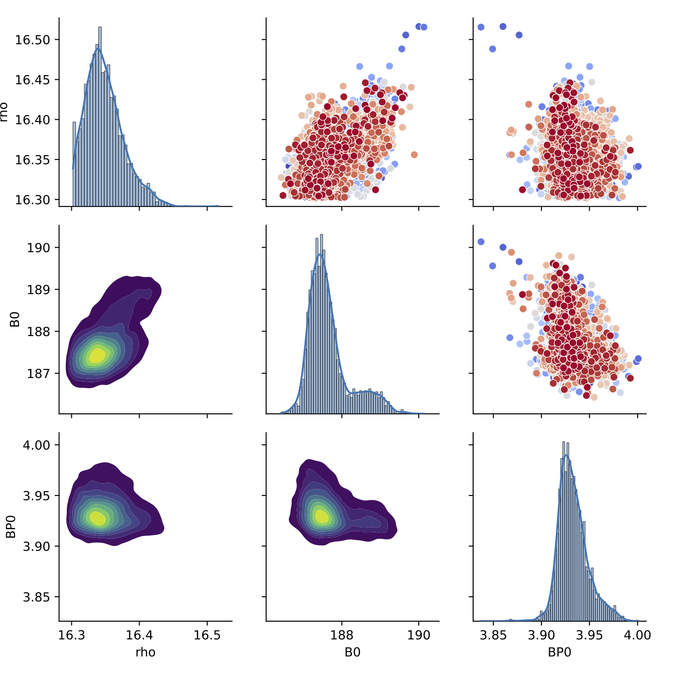
Tantalum Parameters
- With the elastic method we have tighter posteriors over previous methods
- Additionally, scientists at Z have confirmed the parameters conform more to physical understanding of the material
Questions?
jdtuck@sandia.gov