Bayesian Model Calibration
An Elastic Approach
J. Derek Tucker

Sandia National Laboratories
February 24, 2024
Sandia National Laboratories
- Department of Energy National Lab
- 14,000 Staff across 7 Locations
- Two Statistics Departments
- 30 Full Time Staff, 4 Post-Docs, 10 year round interns
![]()
- Collaborators: Devin Francom (LANL), Gabriel Huerta, Kurtis Shuler, Gavin Collins
Outline
- Introduction
- Functional Data Analysis
- Elastic Bayesian Model Calibration
- Results
- Simulation
- Sandia Z-Machine Equation of State
Introduction
- Question: How can we model functions
- Can we use them as predictors in a regression model?
- Can we calibrate a computer model?
- It is the same goal (question) of any area of statistical research
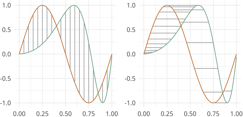
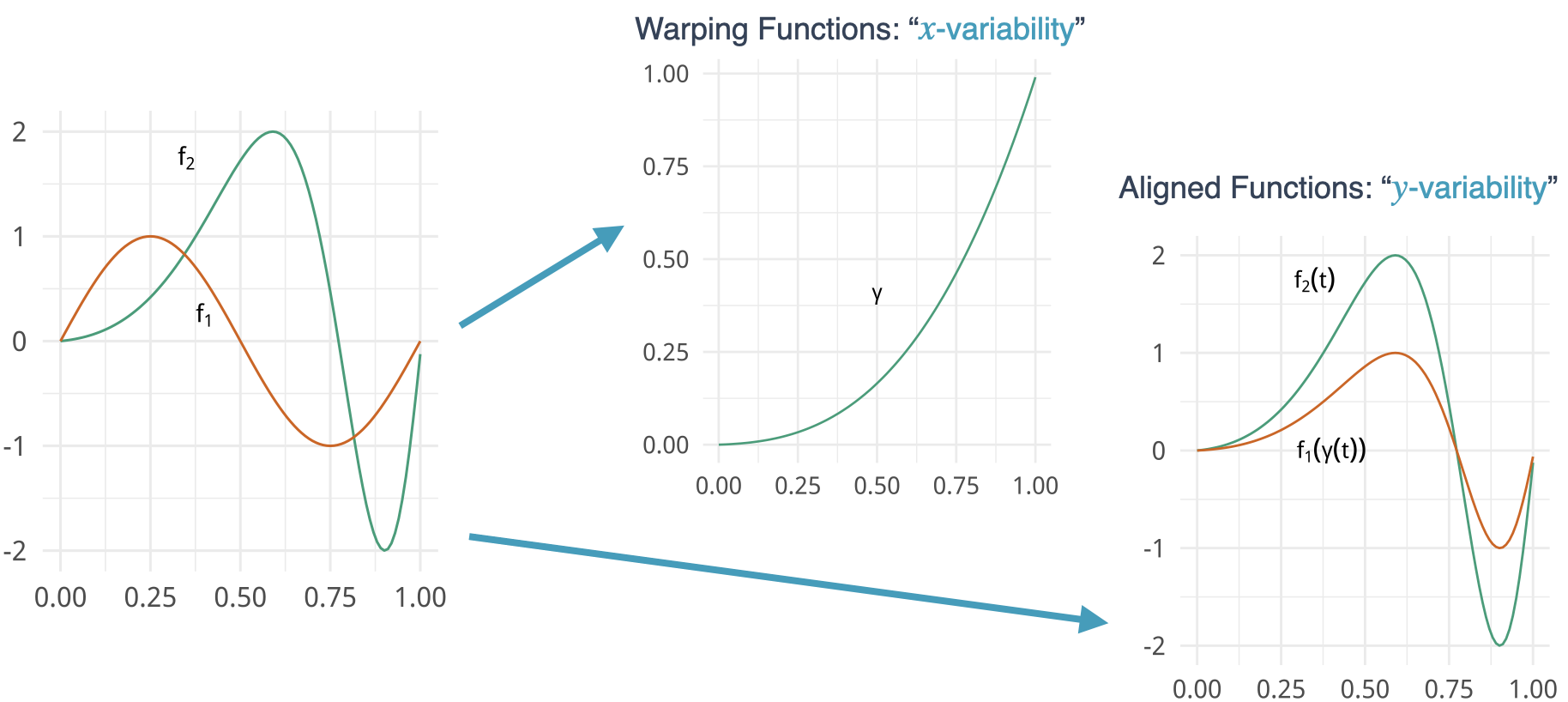
- One problem occurs when performing these types of analysis is that functional data can contain variability in time (x-direction) and amplitude (y-direction)
- How do we characterize and utilize this variability in the models that are constructed from functional data?
FDA versus Multivariate Statistics
In FDA, one develops the theory on function spaces and not finite vectors, and discretizes the function only at the final step – compute implementation
![]()
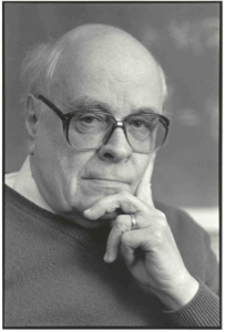
Ulf Grenander: “Discretize as late as possible” (1924-2016)
Even after discretization, we retain the ability to interpolate resample as needed!
Components of Function Variability
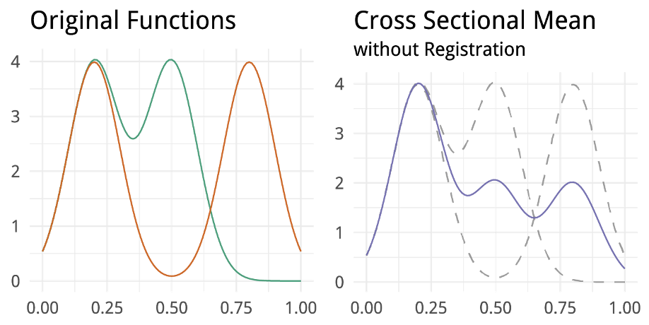
Classical FDA: Loss of Structure
- Cross-sectional statistics ignore horizontal component, often destroys structures
Functional Data Analysis
- Let \(f\) be a real valued-function with the domain \([0,1]\), can be extended to any domain
- Only functions that are absolutely continuous on \([0,1]\)
- Let \(\Gamma\) be the group of all warping functions \[ \Gamma = \{\gamma:[0,1]\rightarrow[0,1]|\gamma(0)=0,\gamma(1)=1,~\gamma \mbox{ is a diffeo}\} \]
- It acts on the function space by composition \[(f,\gamma) = f\circ\gamma\]
- It is common to use the following objective function for alignment \[\min_{\gamma\in\Gamma}\|f_1\circ\gamma-f_2\|\]
- Note: It is not a distance function since it is not symmetric.
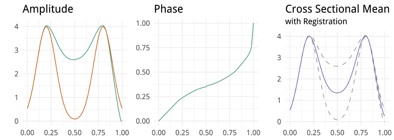
Elastic Distance (Fisher-Rao)
Define the Square Root Velocity Function \[q:[0,1]\rightarrow\mathbb{R}^1,~q(t)=sign(\dot{f}(t))\sqrt{|\dot{f}(t)|}\] Fisher Rao Distance is \(\mathbb{L}^2\) in SRVF space \[d_a(f_1,f_2) = \inf_\gamma\|(q_1\circ\gamma)\sqrt{\dot{\gamma}}-q_2\|\] Distance is a proper distance
Can compute distance on warping functions (how much alignment) \[d_p(\gamma) = \arccos\left(\int_0^1\sqrt{\dot{\gamma}}\,dt\right)\]
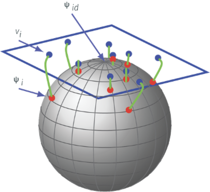
Analysis of \(\Gamma\)
\(\Gamma\) is a nonlinear manifold and it is infinite dimensional
Represent an element of \(\gamma\in\Gamma\) by the square-root of its derivative: \(\psi = \sqrt{\dot{\gamma}}\)
Important advantage of this transformation is the set of all such \(\psi\)’s is a Hilbert Sphere \(\mathbb{S}_\infty\)
Bayesian Model Calibration
- We wish to calibrate a computer model with parameters \(\theta\) to an experiment
- Can compute computer model (simulations) over wide range of \(\theta\)
- The data is functional in nature and has phase and amplitude variability
- Utilize elastic metrics in a Bayesian Model Calibration Framework
Bayesian Model Calibration
Let \(z(t,\boldsymbol{x_i})\) denote an experimental measurement from the \(i^{th}\) experiment
Similarly, let \(y(t,\boldsymbol{x_i}, \boldsymbol{u})\) denote a simulation of the \(i^{th}\) experiment with input parameters \(\boldsymbol{u}\)
An approach to Bayesian model calibration with functional responses is to specify \[z(t,\boldsymbol{x_i}) = y(t,\boldsymbol{x_i},\boldsymbol{\theta}) + \delta(t, \boldsymbol{x_i}) + \epsilon_i(t,\boldsymbol{x_i}), ~~\epsilon(t,\boldsymbol{x_i})\sim \mathcal{N}(0,\sigma_\epsilon^2)\]
Where \(\delta\) is a model discrepancy term and \(\epsilon\) represents all other error
This model will suffer from the aforementioned problems with phase variability
Elastic Bayesian Model Calibration
- Decompose observation into aligned functions and warping functions \[z(t,\boldsymbol{x_i}) = \tilde z(t, \boldsymbol{x_i}) \circ\gamma_{z\rightarrow z}(t,\boldsymbol{x_i})\]
- and decompose the simulations \[y(t,\boldsymbol{x_j}, \boldsymbol{u_j}) = \tilde y(t,\boldsymbol{x_j}, \boldsymbol{u_j}) \circ \gamma_{y\rightarrow z}(t, \boldsymbol{x_j}, \boldsymbol{u_j})\]
- To facilitate modeling, we transform the warping functions into shooting vector space with \[\boldsymbol{v}_{z\rightarrow z}(\boldsymbol{x_i}) = \exp_{\psi}^{-1}\left(\sqrt{\dot\gamma_{z\rightarrow z}(\boldsymbol{x_i})}\right)\] \[\boldsymbol{v}_{y\rightarrow z}(\boldsymbol{x_j},\boldsymbol{u_j}) = \exp_{\psi}^{-1}\left(\sqrt{\dot\gamma_{y\rightarrow z}(\boldsymbol{x_j},\boldsymbol{u_j})}\right)\]
Elastic Bayesian Model Calibration
- Calibrate the aligned data and shooting vectors using the following model \[\tilde{z}(t,\boldsymbol{x_i}) = \tilde{y}(t, \boldsymbol{x_i}, \boldsymbol{\theta}) + \delta_{\tilde{y}}(t, \boldsymbol{x_i}) + \epsilon_{\tilde{z}}(t, \boldsymbol{x_i}), ~~\epsilon_{\tilde{z}}(t, \boldsymbol{x_i})\sim \mathcal{N}(0,\sigma_{\tilde{z}}^2)\] \[\boldsymbol{v}_{z\rightarrow z}(\boldsymbol{x_i}) = \boldsymbol{v}_{y\rightarrow z}(\boldsymbol{x_i}, \boldsymbol{\theta}) + \boldsymbol{\delta_v(\boldsymbol{x_i})} + \boldsymbol{\epsilon_v(\boldsymbol{x_i})}, ~~\boldsymbol{\epsilon_v(\boldsymbol{x_i})} \sim \mathcal{N}(0,\sigma_v^2\boldsymbol{I})\]
- Note: The shooting vector will be identity if the data is aligned to the observation (experiment)
- Then if \(\theta\) is calibrated correctly the shooting vectors will be identity
MCMC Sampling
For each experiment the likelihood is a Gaussian likelihood
- We fit an emulator (Gaussian Process, BASS, MARS) to the simulated data
- Uniform priors on \(\theta\)
- Sample posterior using delayed rejection adaptive Metropolis Hastings
- Implemented using Impala (LANL) or Dakota (SNL) calibration framework
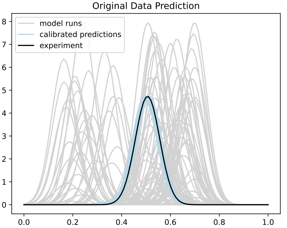
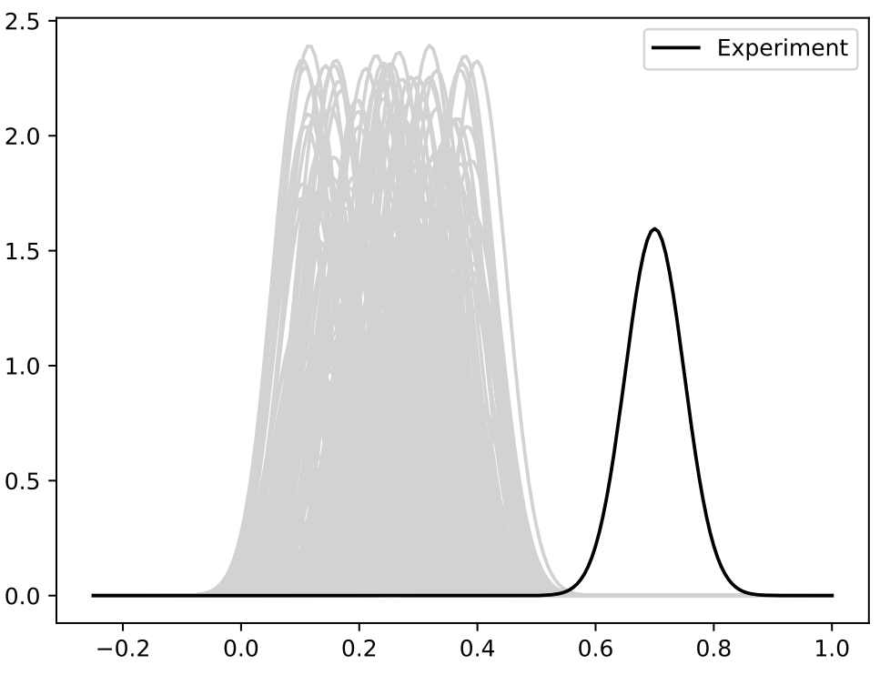
Simulation
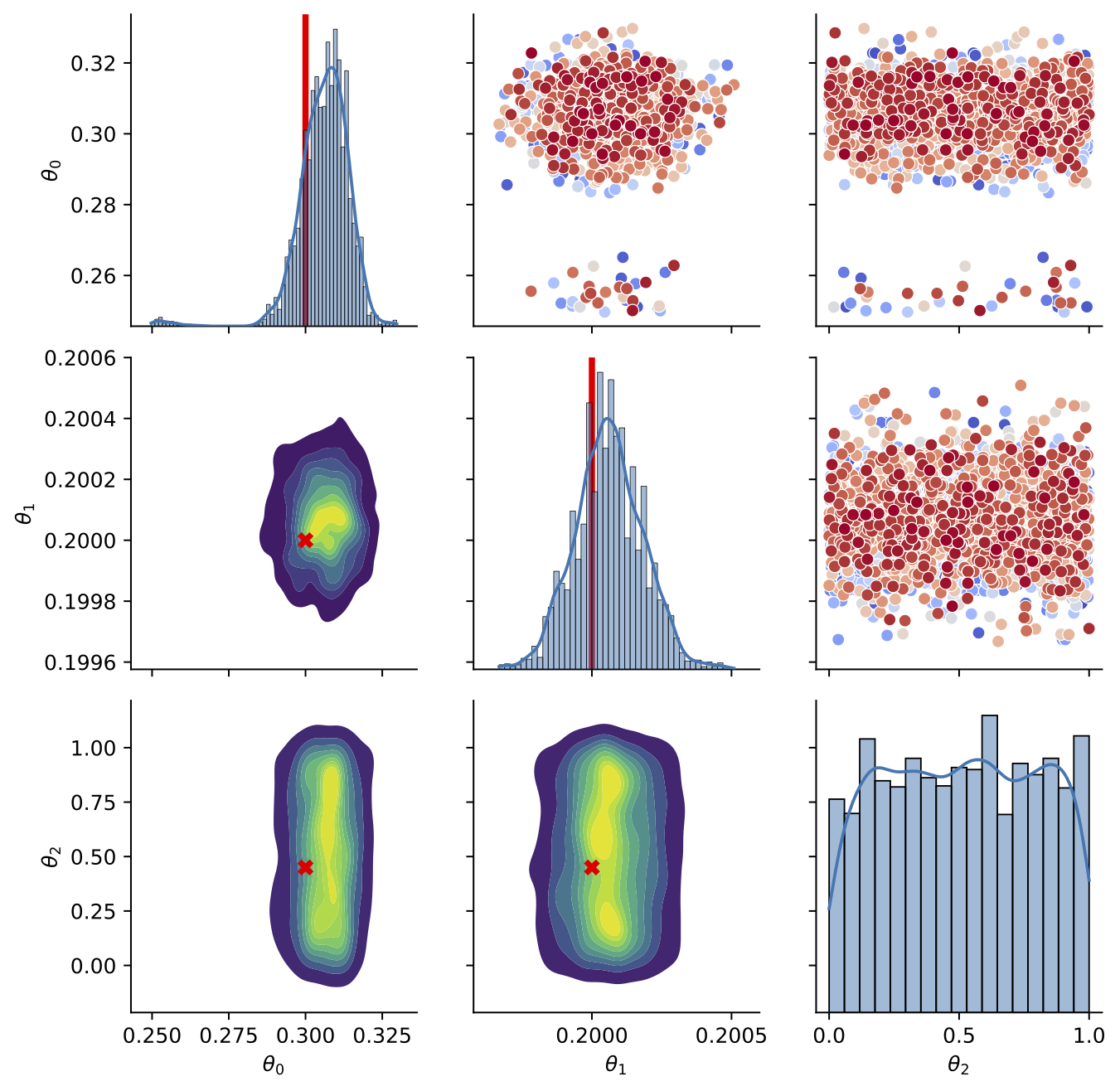
- Simulation study where each function is parameterized Gaussian pdf
- A set of 100 functions were simulated with \(\theta_0,\theta_1\) being drawn from a \(U[0,1]\)
- Third nuisance parameter \(\theta_2\) also drawn from \(U[0,1]\)
\[f_i(t) = \frac{\theta_1}{0.05\sqrt{2\pi}}\exp\left(-\frac{1}{2}\left(\frac{t-(\sin(2\pi \theta_0^2)/4-\theta_0/10+0.5)}{0.05}\right)^2\right)\]
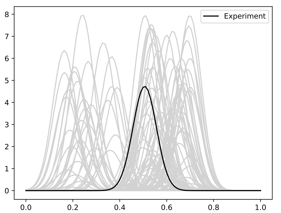
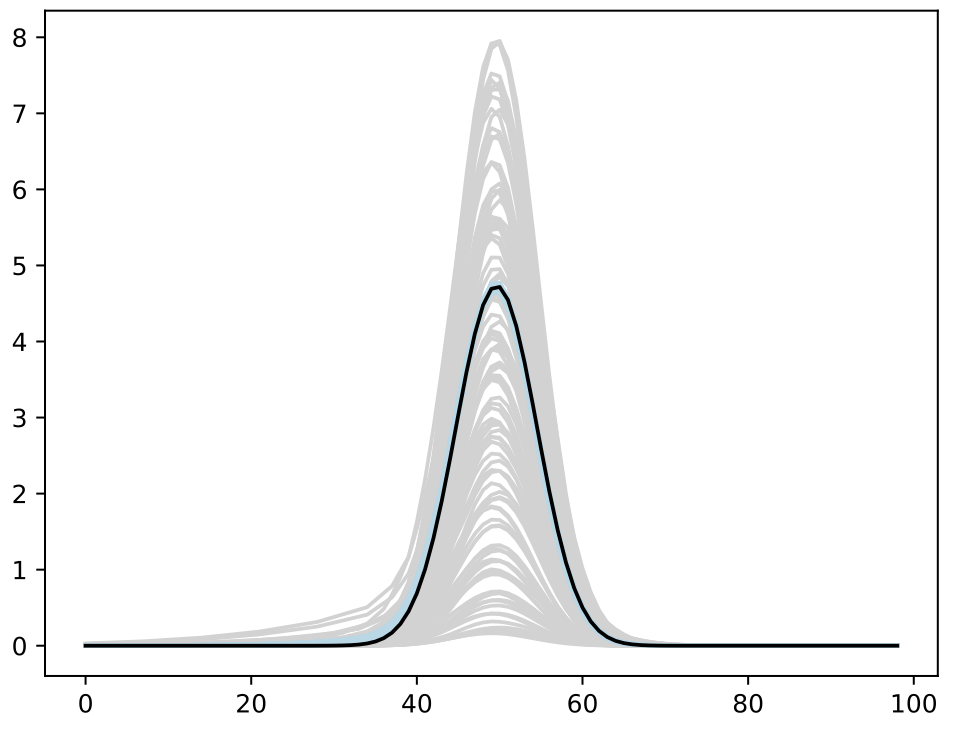
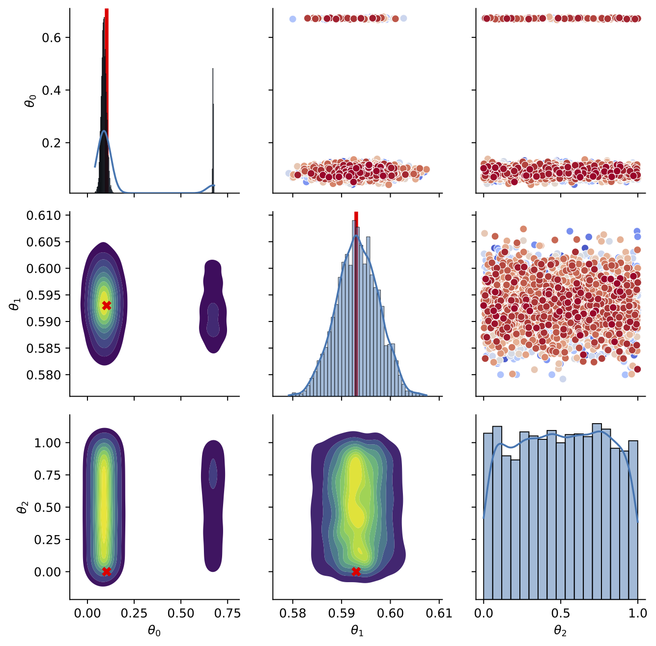
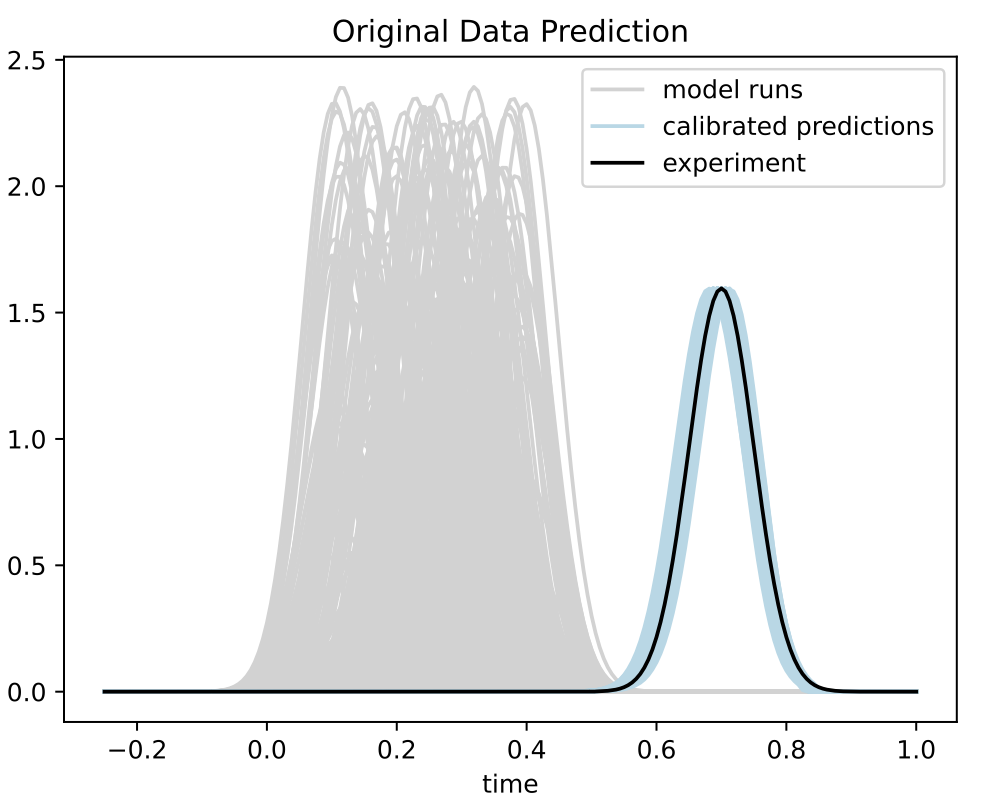
Calibration
- Trained BASS Emulator on Aligned Functions and Shooting Vectors (using elastic fPCA)
- Calibrated using framework with tempering and adaptive MCMC
- Blue shows draws from posterior distribution at 95% credible interval
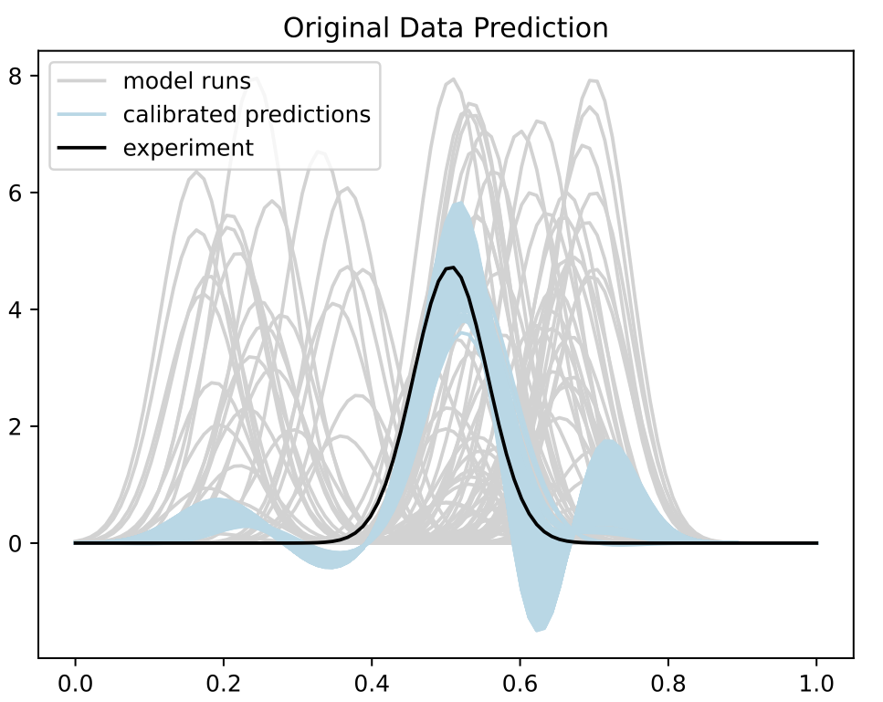
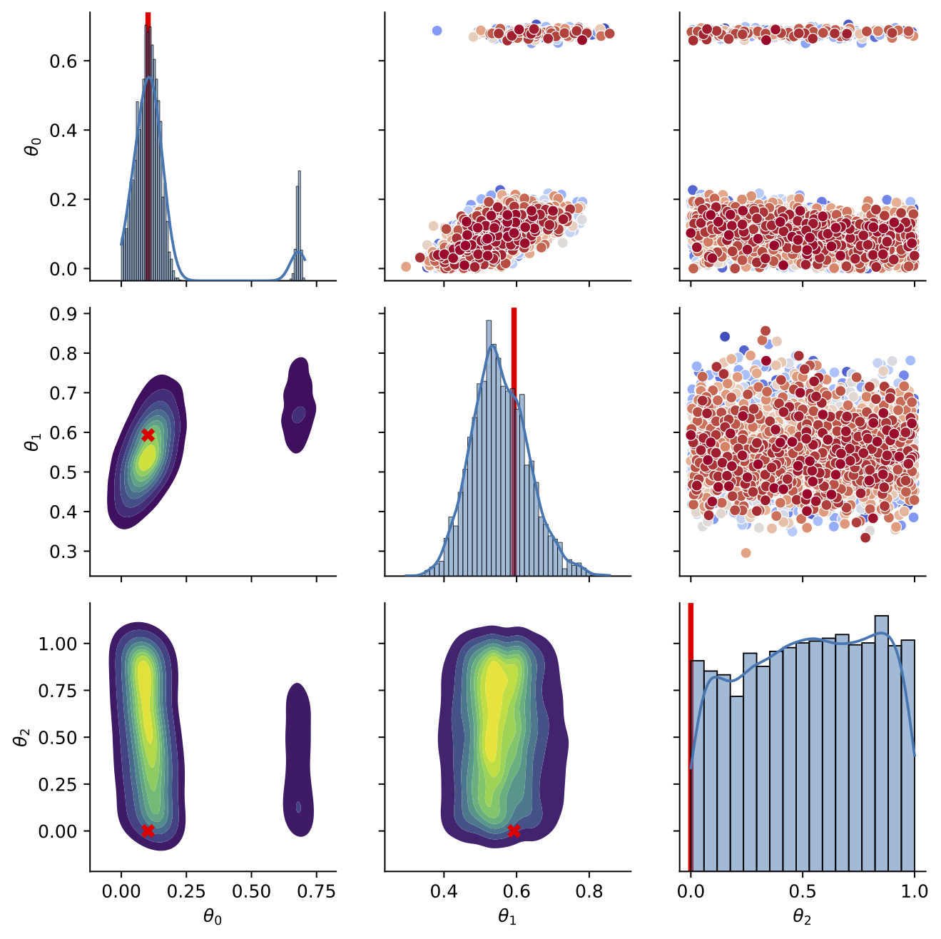
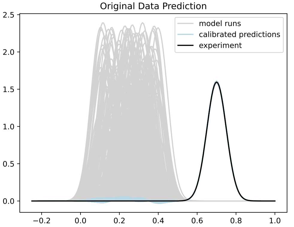
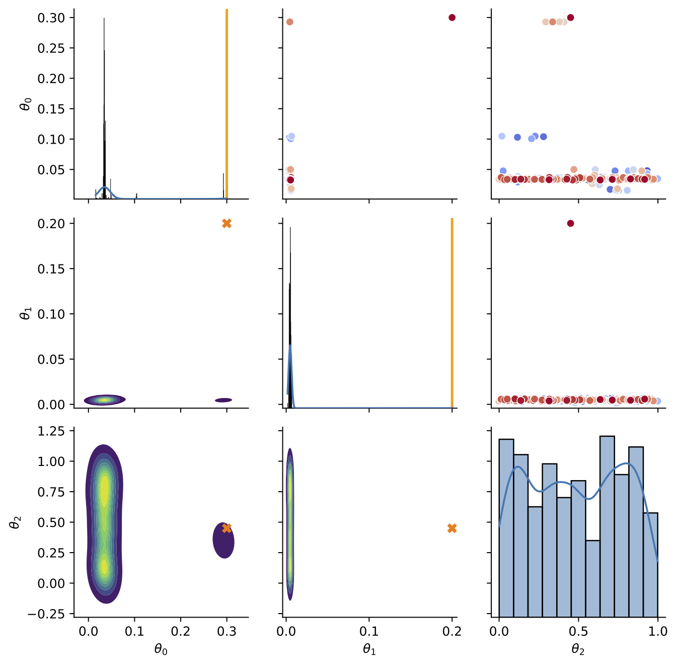
Comparison to Standard Method
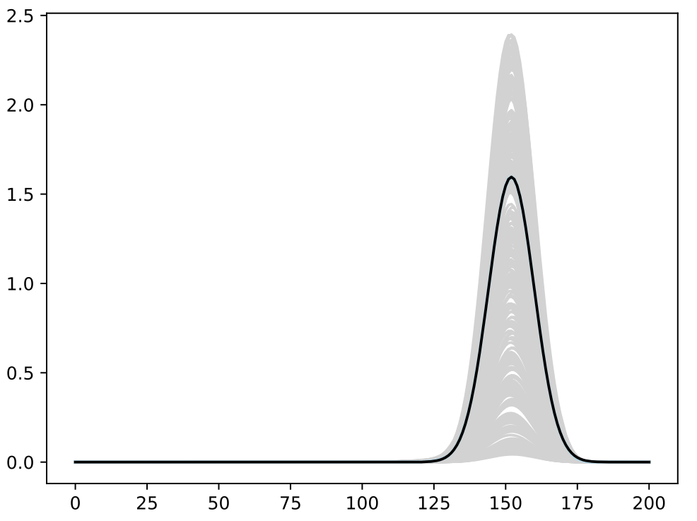
Simulation with Discrepancy
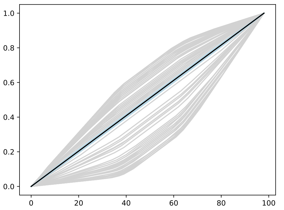
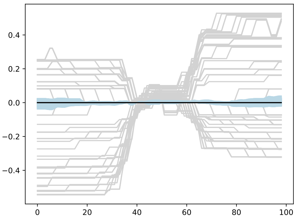
- Repeat same simulation model with with the experiment having a timing discrepancy
- Discrepancy modeling with basis functions in shooting vector space
Calibration
- Trained BASS Emulator on Aligned Functions and Shooting Vectors (using elastic fPCA)
- Calibrated using framework with tempering and adaptive MCMC
- Blue shows draws from posterior distribution at 95% credible interval
Comparison to Standard Method
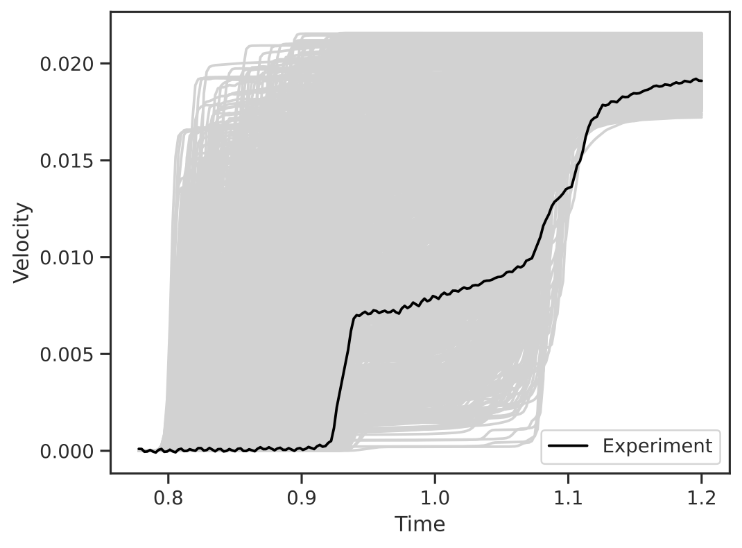
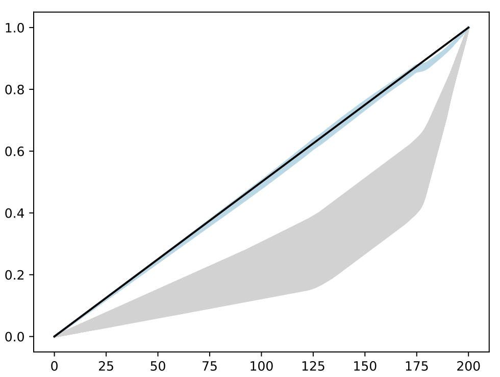
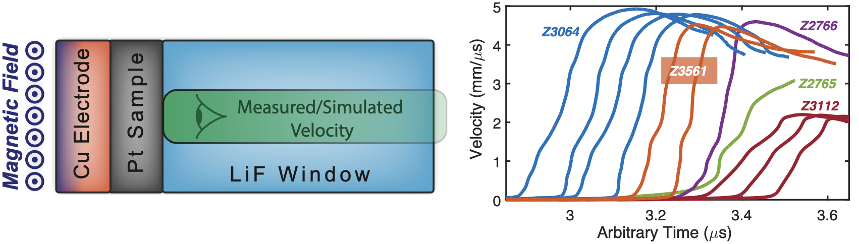
Calibration of Platinum Equation of State
![]()
Calibration equation of state of platinum generated with pulse magnetic fields
Estimate the parameters describing the compressibility (relationship between pressure and density) to understand extreme pressures
Conducted using Sandia Z-machine, a pulse power drive reactor
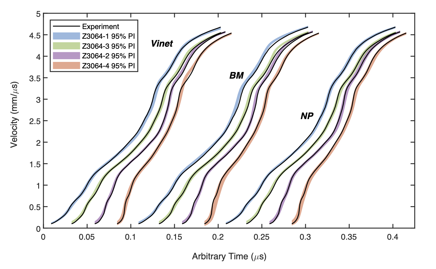
Calibration
![]()
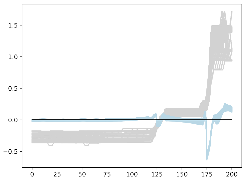
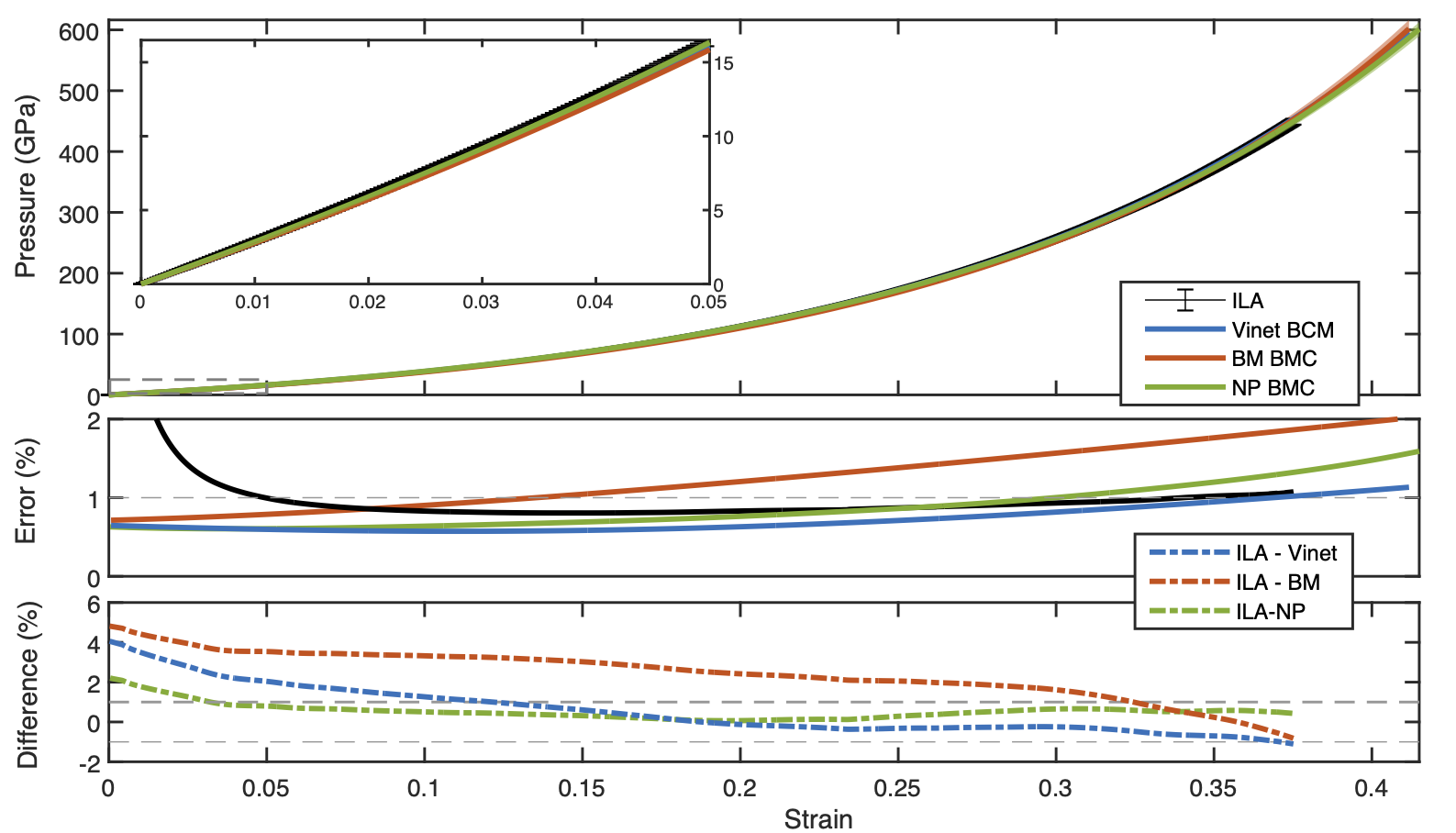
Comparison to ILA
Comparison to numerical method (ILA), we have good agreement
Small percentage difference between ILA and Calibrated Model
![]()
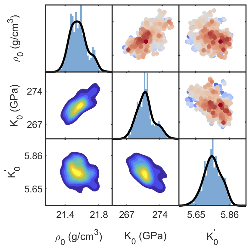
Platinum Parameters
With the elastic method we have tighter posteriors over previous methods
Additionally, scientists at Z have confirmed the parameters conform more to physical understanding of the material
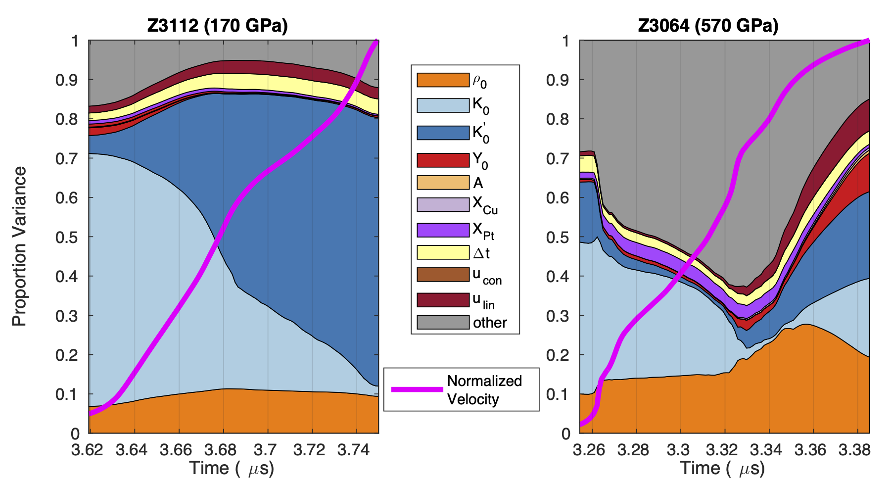
Sensitivity Analysis
![]()
Summary
Functional metrics provide a global measure of the difference of a function in terms of amplitude and phase
Integrated elastic functional metrics into Bayesian Model Calibration framework utilizing aligned data and shooting vector representation
Demonstrated ability on simulated and platinum equation of state calibration problems
Future Work
- Additional testing on real world examples
Papers
D. Francom, J. D. Tucker, J. G. Huerta, K. Shuler, and D. Ries, “Elastic Bayesian Model Calibration”, arXiv:2305.08834 [stat.ME], in revision, 2023.
J. Brown, J. P. Davis, J. D. Tucker, J. G. Huerta, and K. Shuler, “Quantifying uncertainty in analysis of shockless dynamic compression experiments on platinum, Part 2: Bayesian model calibration”, Journal of Applied Physics, vol. 134, no. 23, 2023.
Questions?
jdtuck@sandia.gov
http://research.tetonedge.net